Verteilungsbasiert vs. simulationsbasiert
Verteilungsannahmen
... können falsch sein
Rousselet, G. A., Pernet, C. R., & Wilcox, R. R. (2019). A practical introduction to the bootstrap: A versatile method to make inferences by using data-driven simulations [Preprint]. PsyArXiv. https://doi.org/10.31234/osf.io/h8ft7
Der t-Test bei schiefen Verteilungen (I/II)
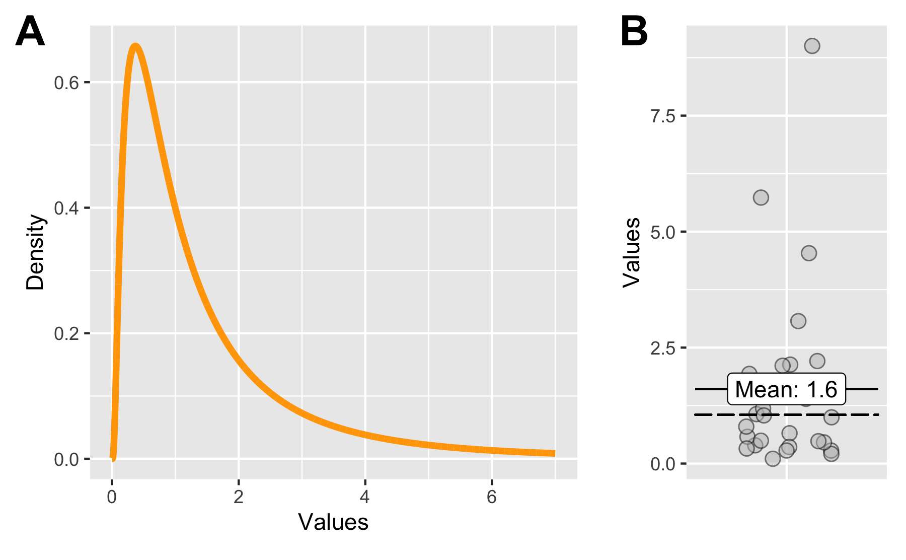
95%-KI auf Basis der der t-Verteilung mit 29 df:
#> [1] 0.9037929 2.3149338#> attr(,"conf.level")#> [1] 0.95Der t-Test bei schiefen Verteilungen (II/II)
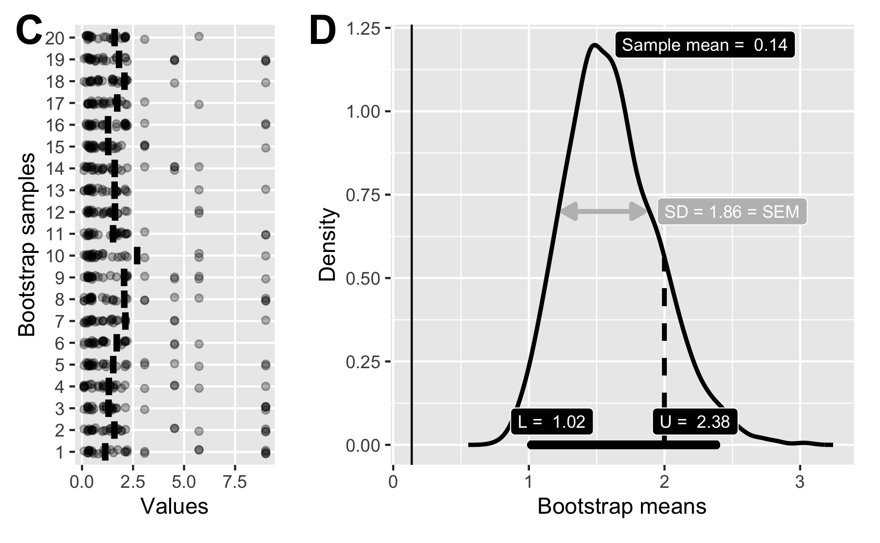
Rousselet, G. A., Pernet, C. R., & Wilcox, R. R. (2019). A practical introduction to the bootstrap: A versatile method to make inferences by using data-driven simulations [Preprint]. PsyArXiv. https://doi.org/10.31234/osf.io/h8ft7
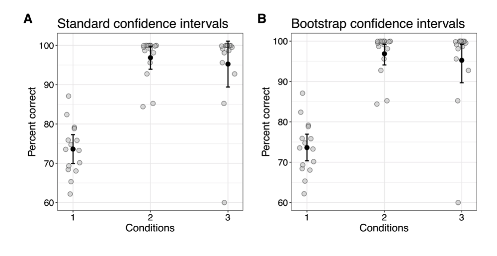
Simulationstechniken sind nicht per se robuster
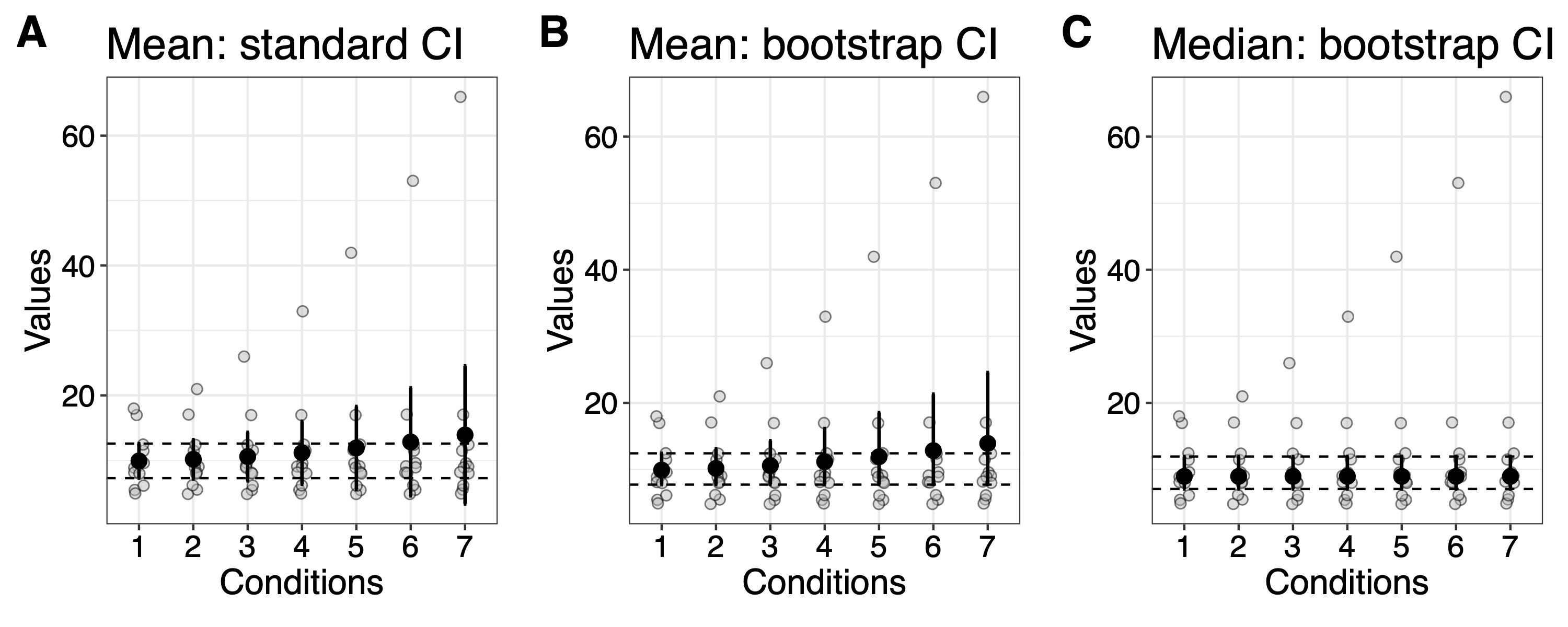
Rousselet, G. A., Pernet, C. R., & Wilcox, R. R. (2019). A practical introduction to the bootstrap: A versatile method to make inferences by using data-driven simulations [Preprint]. PsyArXiv. https://doi.org/10.31234/osf.io/h8ft7
Repro-Krise?
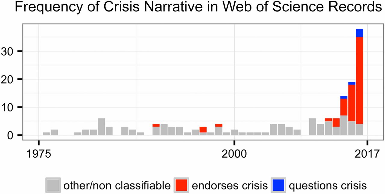
Fanelli, D. (2018). Opinion: Is science really facing a reproducibility crisis, and do we need it to? Proceedings of the National Academy of Sciences, 115(11), 2628–2631. https://doi.org/10.1073/pnas.1708272114
Du hast die Wahl

Im Rahmen des normalen Unterrichts einer Sonderveranstaltung der FOM wurde der Versuch durchgeführt:
- \(n=34\) Versuchspersonen*
- \(x=12\) Treffer
* Selbstloser Einsatz für die Wissenschaft
Ablauf: Schmeck den Pringel heraus!
Je zwei Personen, \(A\) und \(B\) finden sich in Pärchen
\(A\) wählt 1 Pringel-Chip und 2 Noname-Chips
\(A\) reicht \(B\) nacheinander die 3 Chips in zufälliger Reihenfolge, \(B\) hat dabei die Augen geschlossen
\(B\) entscheidet sich, welcher Chips vermutlich der Pringle-Chip ist
Das Ergebnis (Treffer ja/nein) kann hier eingetragen werden: https://forms.gle/w1bUMGvdDofadih68
Bitte notieren Sie das Ergebnis (Treffer ja/nein) auch auf einen Zettel (den zusammenfalten)
Barcode zum Link:

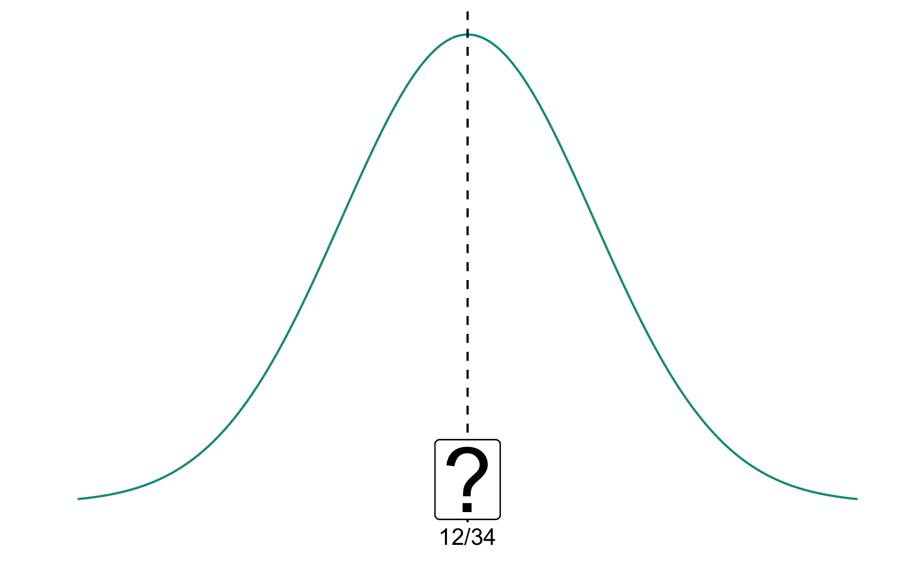
Was ist der wahre Erschmecker-Anteil?
Anteil Stichprobe: 12/34
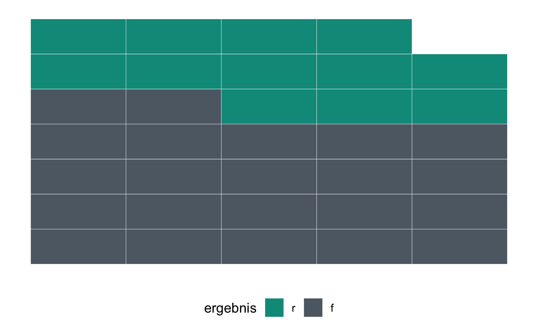
Anteil in Population der FOM-Profs???
Idee 1: Wir testen alle FOM-Profs!

super. Dauert aber.
Idee 2: Wir wiederholen der Versuch oft!
z.B. 100 Mal:
super. Dauert aber.
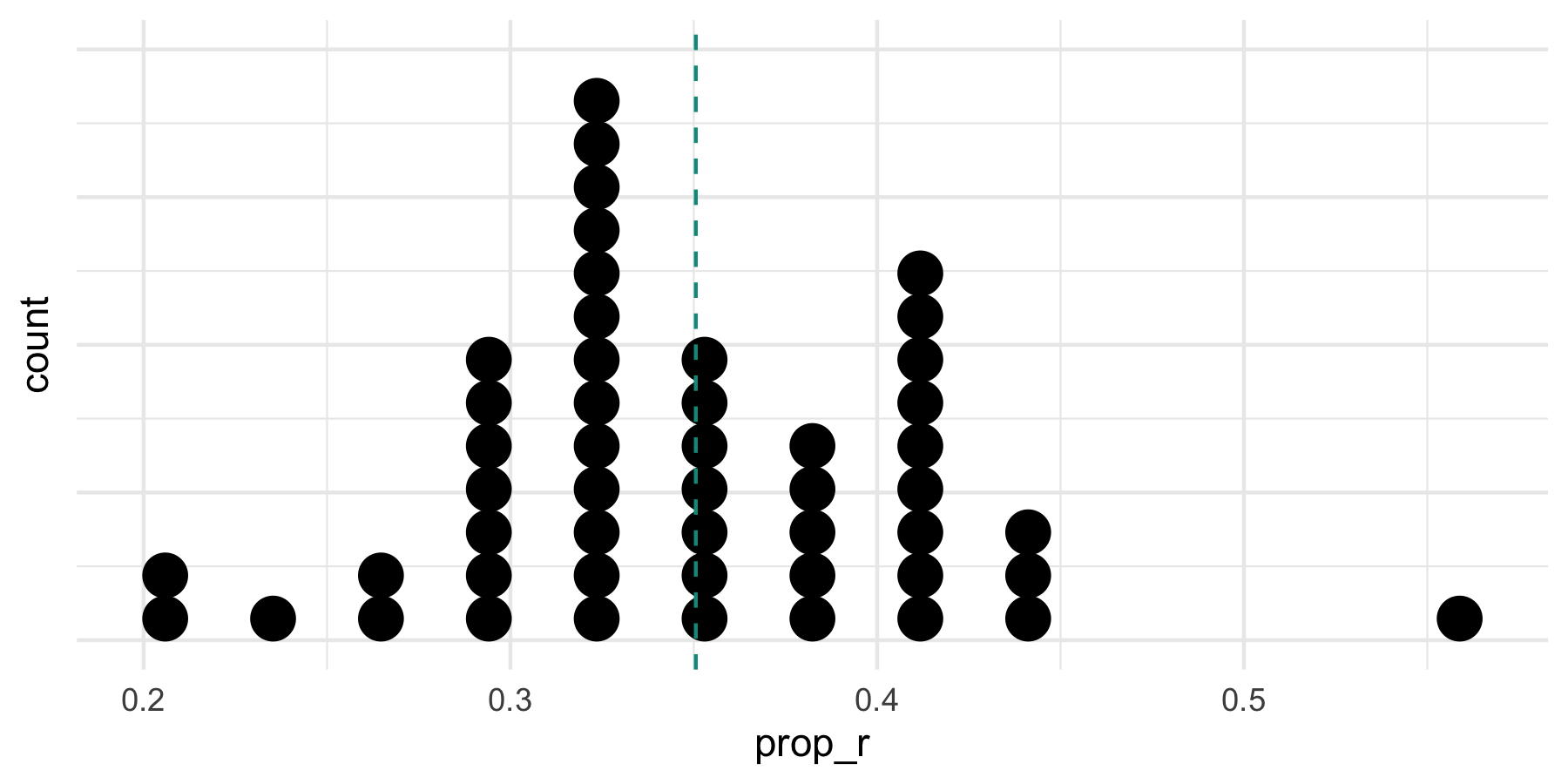
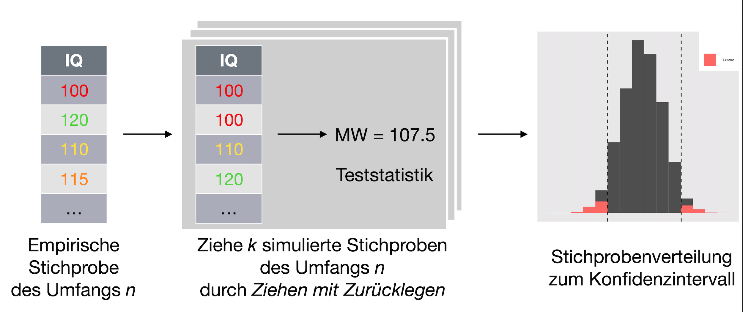
Idee 3: Der Münchhausen-Trick
Ziele viele Stichproben mit Zurücklegen
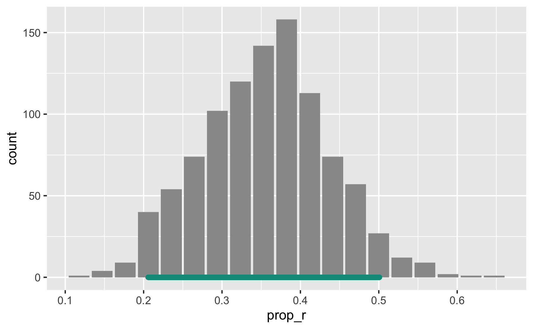
Voila -- Die Bootstrap-Verteilung:
Auf Errisch geht das so...
library(mosaic)# unsere Stichprobe:stipro <- rep(factor(c("f","r")), c(22, 12)) # 3 Bootstrap-Stichproben:boot1 <- mosaic::do(3) * prop( ~ resample(stipro), success = "r") boot1#> prop_r#> 1 0.3529412#> 2 0.3823529#> 3 0.3529412# Histogramm zeichnen:gf_bar( ~ prop_r, data = Bootvtlg)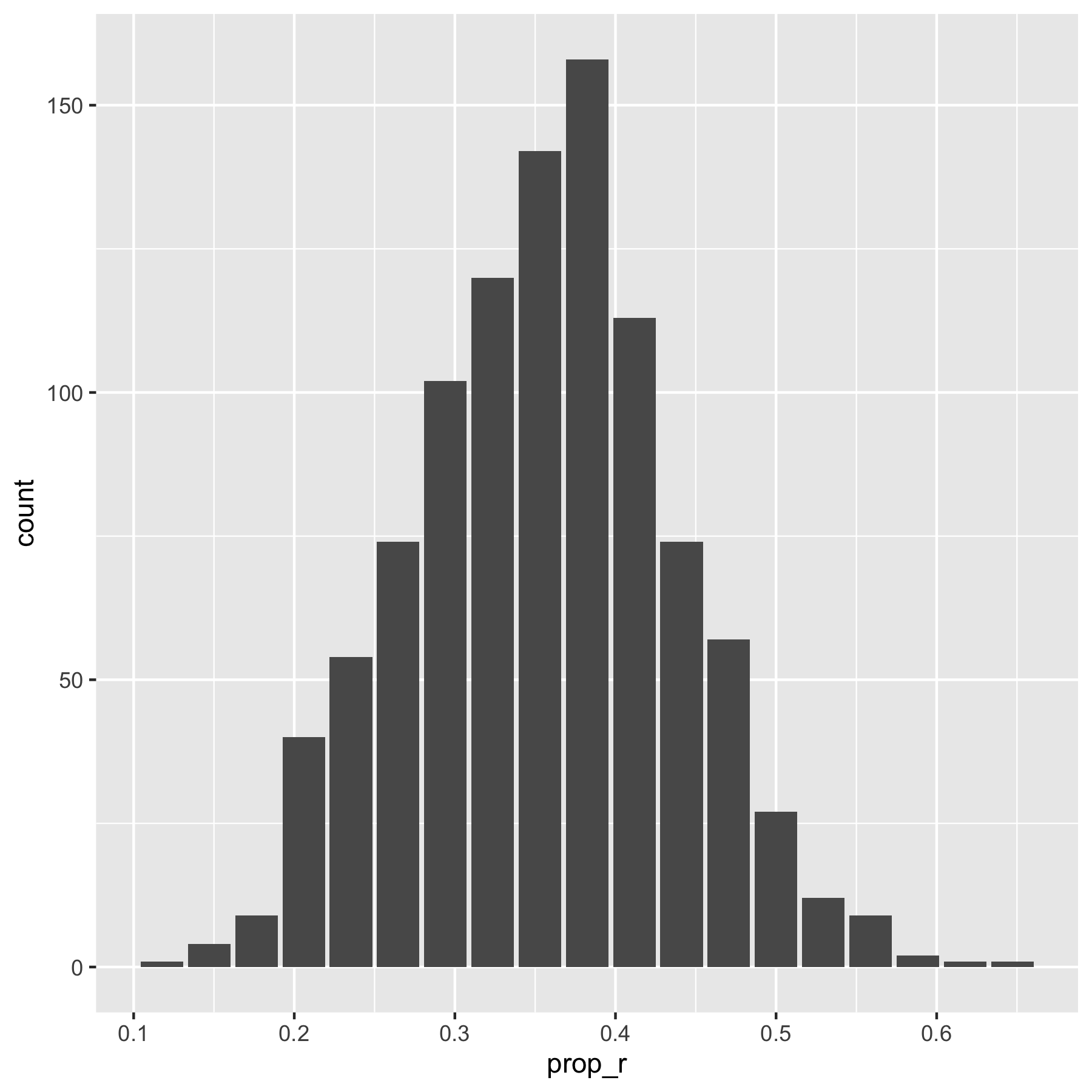
Wir erzeugen 1000 Rate-Stichproben
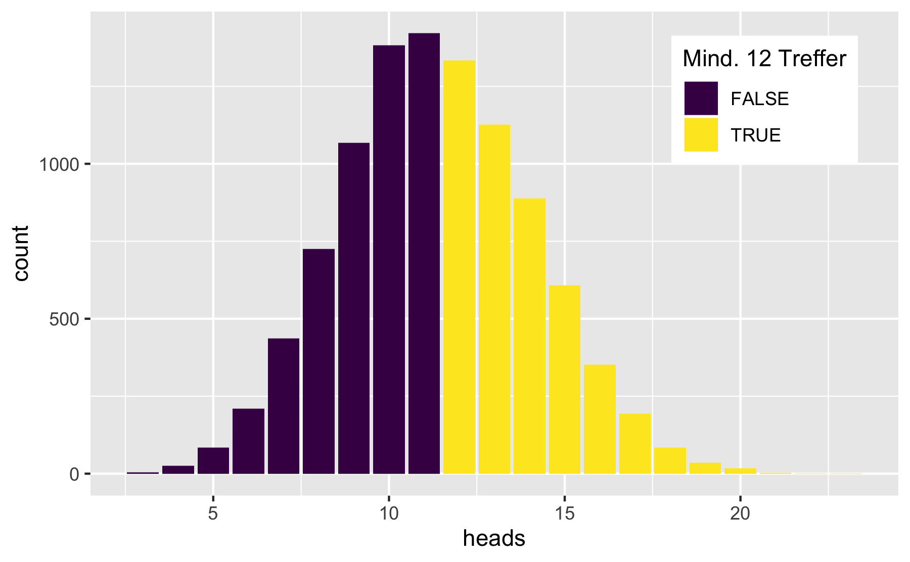
Nullvtlg <- mosaic::do(10000) * rflip(n = 34, prob = 1/3)gf_bar( ~ heads, data = Nullvtlg )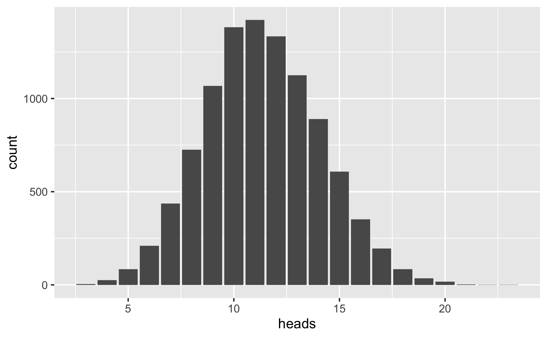
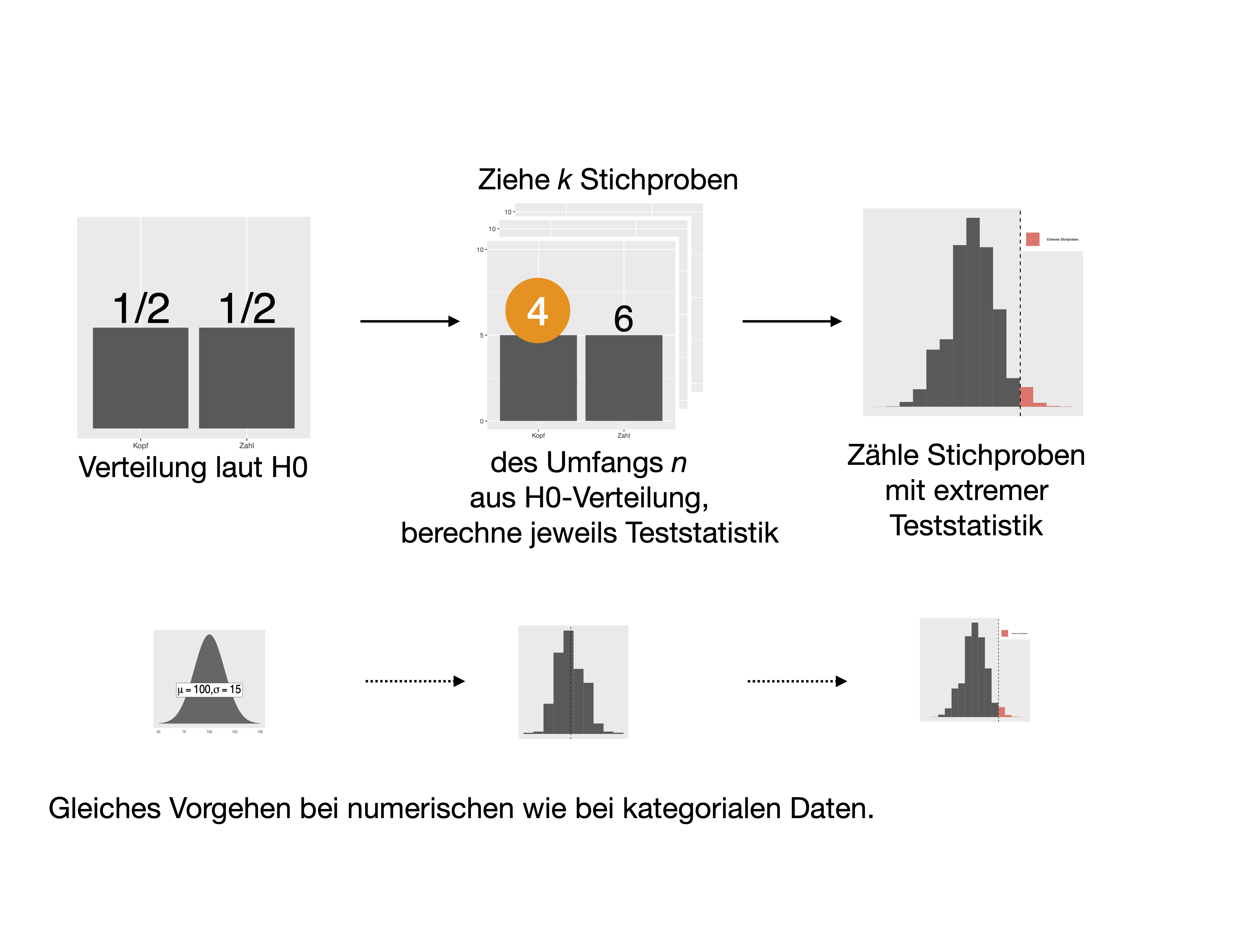
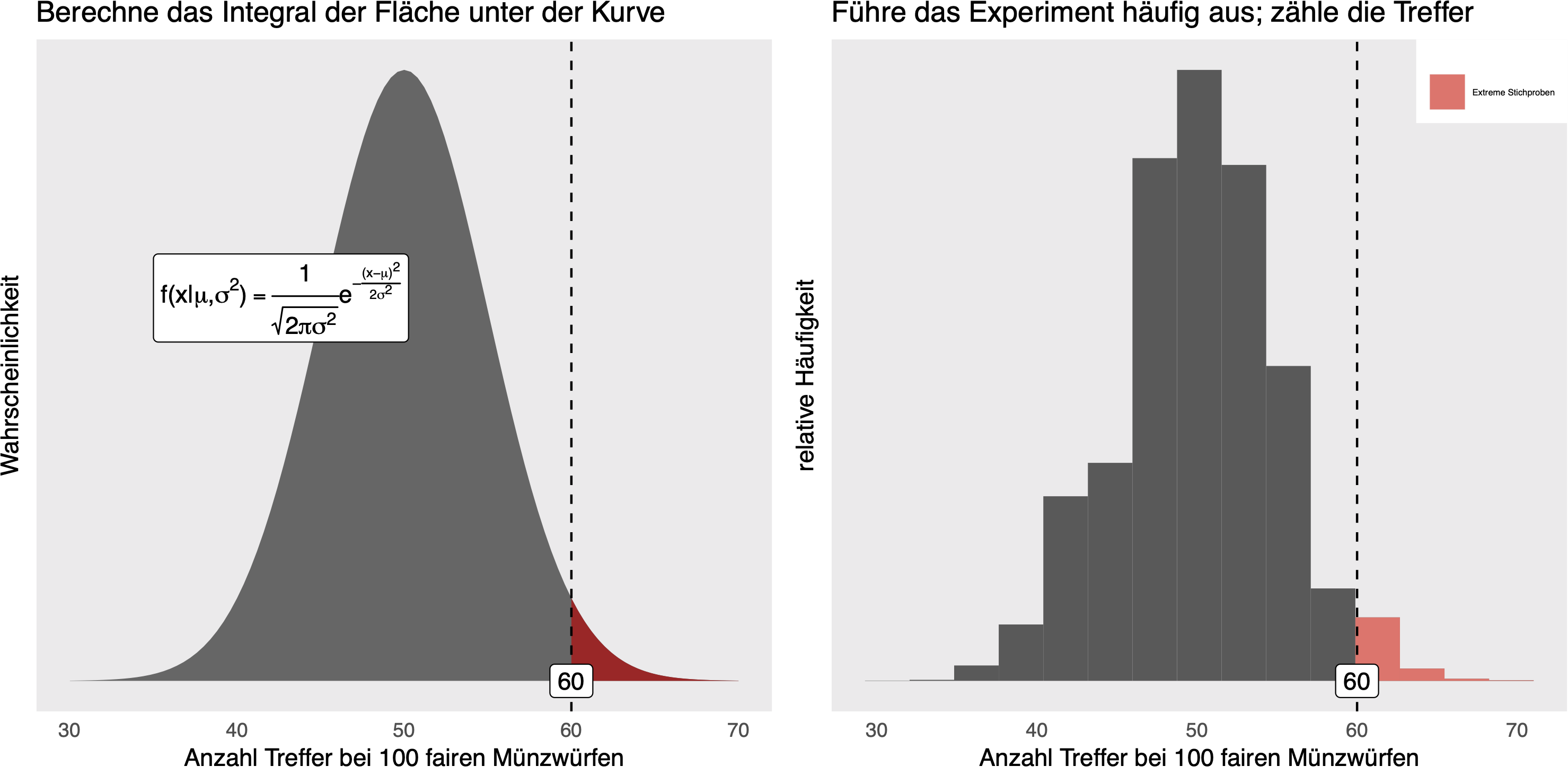
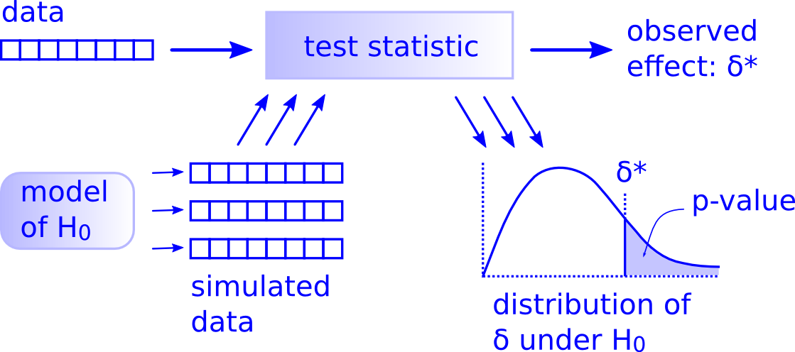
Die Blaupause eines (jeden) statistisches Tests
p-Wert
p-Wert: Anteil der Stichproben mit mindestens 12 Treffer:
gf_bar( ~ heads, data = Nullvtlg)
prop( ~ heads >= 12, data = Nullvtlg)#> prop_TRUE #> 0.4644Als sehr, sehr wichtig

... wird der p-Wert von vielen erachtet.
Die Daten sind plausibel unter der Nullhypothese.
Die Daten sind mit der \(H_0\) kompatibel.
Wir können die Nullhypothese also nicht ablehnen.
p-Wert: Eine gute Geschichte
... verdient, aufgebauscht zu werden (?)
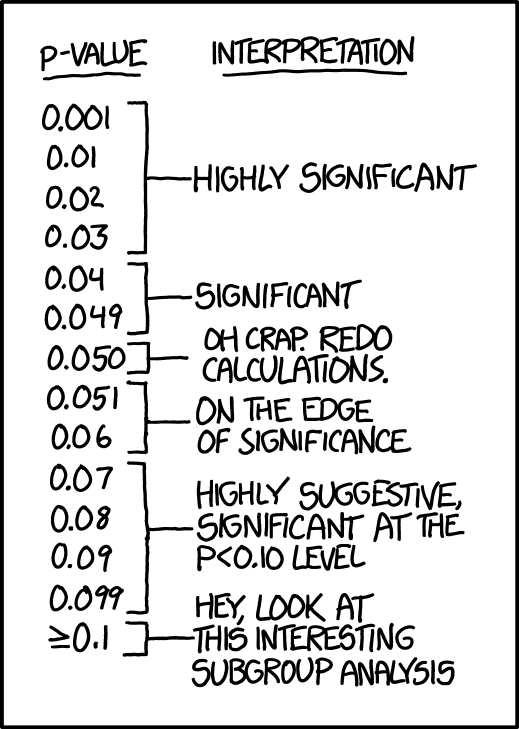
www.xkcd.com/about Note: You are welcome to reprint occasional comics pretty much anywhere (presentations, papers, blogs with ads, etc). If you're not outright merchandizing, you're probably fine. Just be sure to attribute the comic to xkcd.com.
Forschung über dem 5%-Niveau

"... some statisticians prefer to supplement or even replace p-values with other approaches. These include methods that emphasize estimation over testing, such as confidence ... intervals ..."
"Good statistical practice ... emphasizes principles of good study design ... , a variety of numerical and graphical summaries of data, understanding of the phenomenon under study, interpretation of results in context, complete reporting and proper logical and quantitative understanding of what data summaries mean."
... No single index should substitute for scientific reasoning.
Ronald L. Wasserstein & Nicole A. Lazar (2016) The ASA Statement on p-Values: Context, Process, and Purpose, The American Statistician, 70:2, 129-133, DOI: 10.1080/00031305.2016.1154108
Stimmt Lächeln nachsichtiger?

Skeptiker:
"Lächeln bringt doch nichts!"
\(H_0: \mu_{\text{Lächeln}} \le \mu_{\text{Neutral}}\)
\(H_A: \mu_{\text{Lächeln}} > \mu_{\text{Neutral}}\)
LaFrance, M., & Hecht, M. A. (1995). Why smiles generate leniency. Personality and Social Psychology Bulletin, 21(3), 207-214, https://doi.org/10.1177%2F0146167295213002
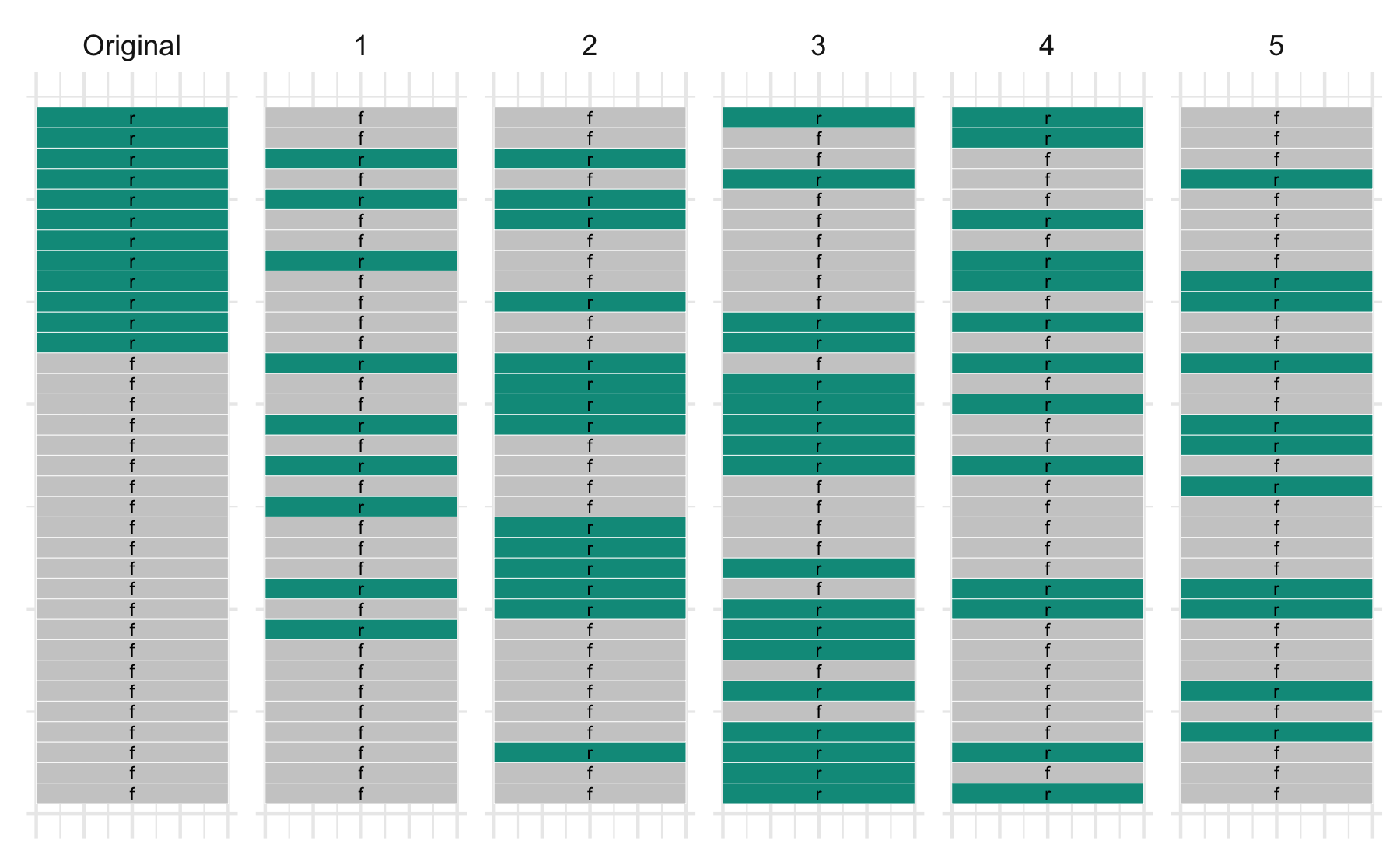
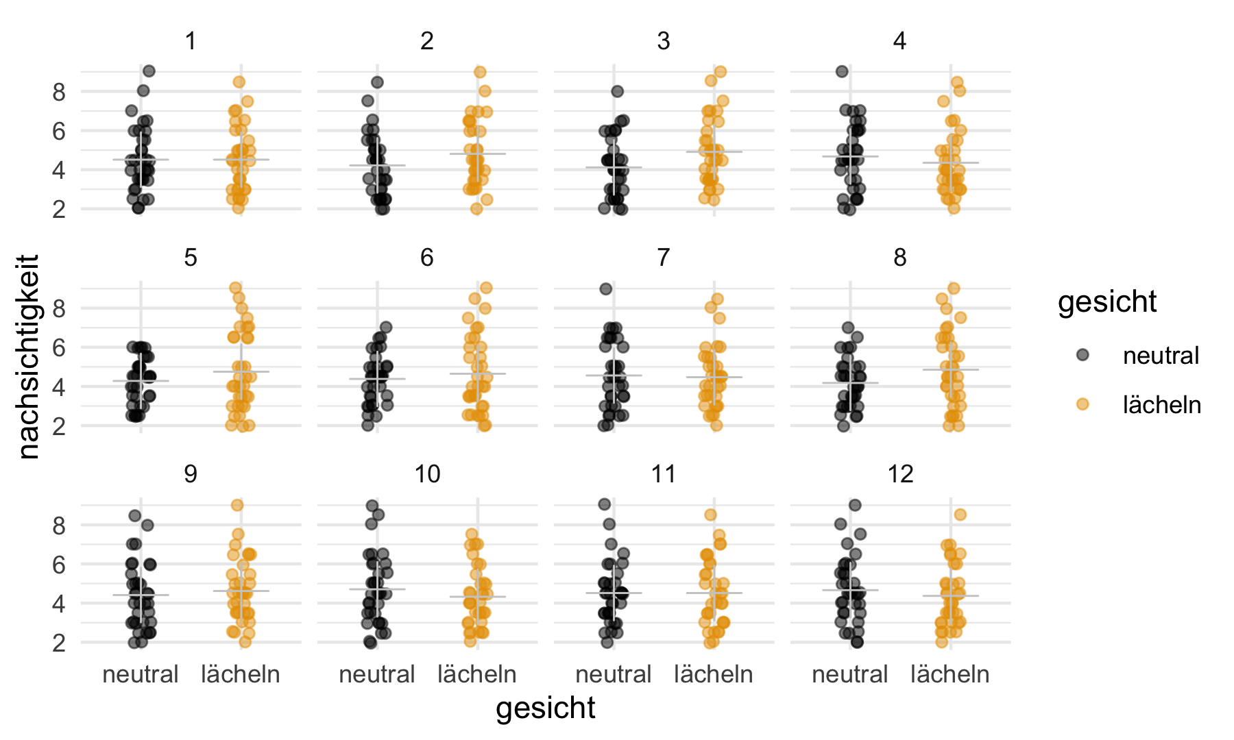
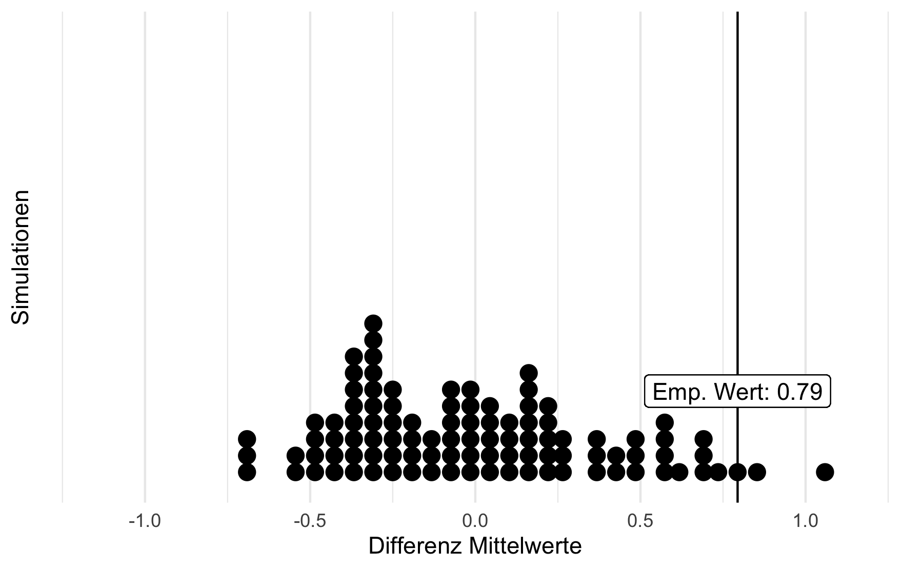
Finde den echten Datensatz
11 Datensätze wurden so simuliert, dass es keinen Unterschied in den Mittelwerten der Populationen gibt, 1 Datensatz ist echt.
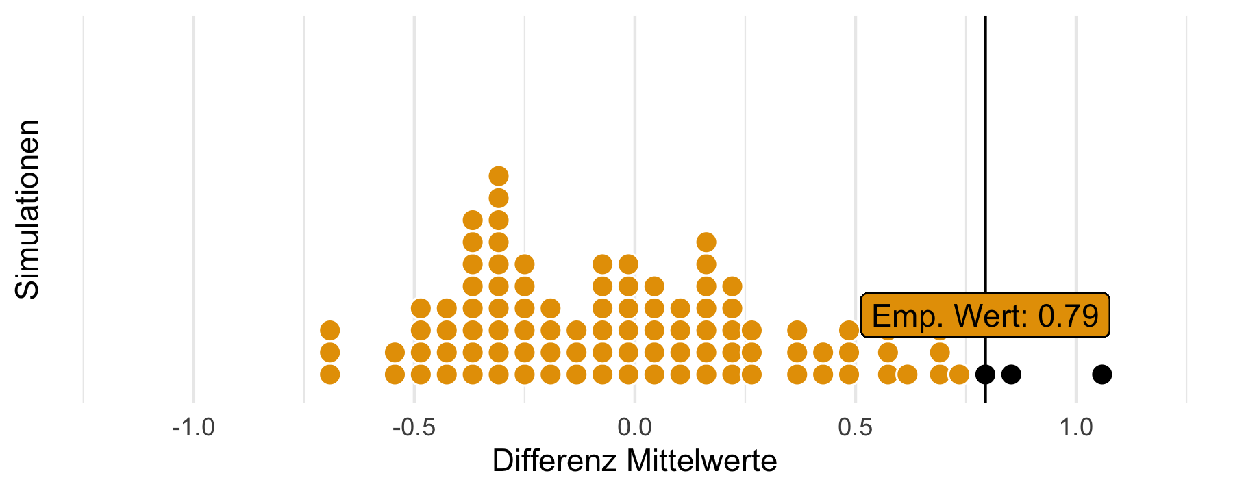
Angenommen, es gäbe keinen Zusammenhang
... von Lächeln und Nachsichtigkeit. Wie häufig wäre unser empirischer Wert in diesen Stichproben?
Der p-Wert schlägt zurück
Wenn die Daten aus einer Population stammen, in der die Nullhypothese stimmt, dann ist unser empirisches Ergebnis selten (unplausibel).
Auf dieser Basis entscheiden wir uns in diesem Fall, die \(H_0\) zu verwerfen (bzw. nicht mehr so stark wie vorher an sie zu glauben).
Wie stellt man die Nullverteilung her?
1.
Man reist in ein Land, in dem es keinen Zusammenhang gibt (zwischen Lächeln und Nachsichtigkeit) und zieht dort viele Stichproben.
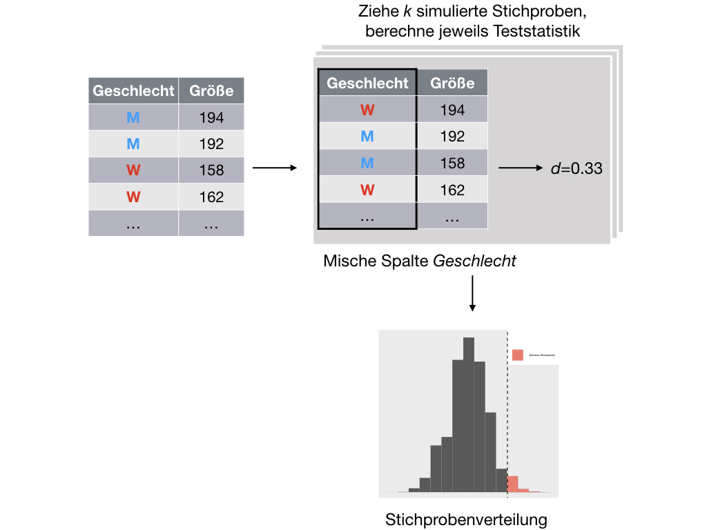
... Oder man mischt eine Spalte
2.
Man mischt die Spalte (z.B. UV) durch, so dass der Zusammenhang zwischen der Spalte UV under einer anderen Spalte (AV) aufgelöst wird.
Übung: Konsumieren Raucher im Schnitt mehr? (2/3)
\(H_0\)-Verteilung visualisieren:
gf_histogram( ~ diffmean, data = Nullvtlg_Raucher) %>%gf_vline(xintercept = ~diffmean(total_bill ~ smoker, data = tips))
Übung: Konsumieren Raucher im Schnitt mehr? (2/3)
Empirische Differenz/Wert in der Stichprobe:
#> diffmean #> 1.568066Anteil der Stichproben, die mind. so groß sind wie der emp. Wert:
#> prop_TRUE #> 0.099Mal zwei nehmen, da ungerichtete Hypothese:
#> prop_TRUE #> 0.198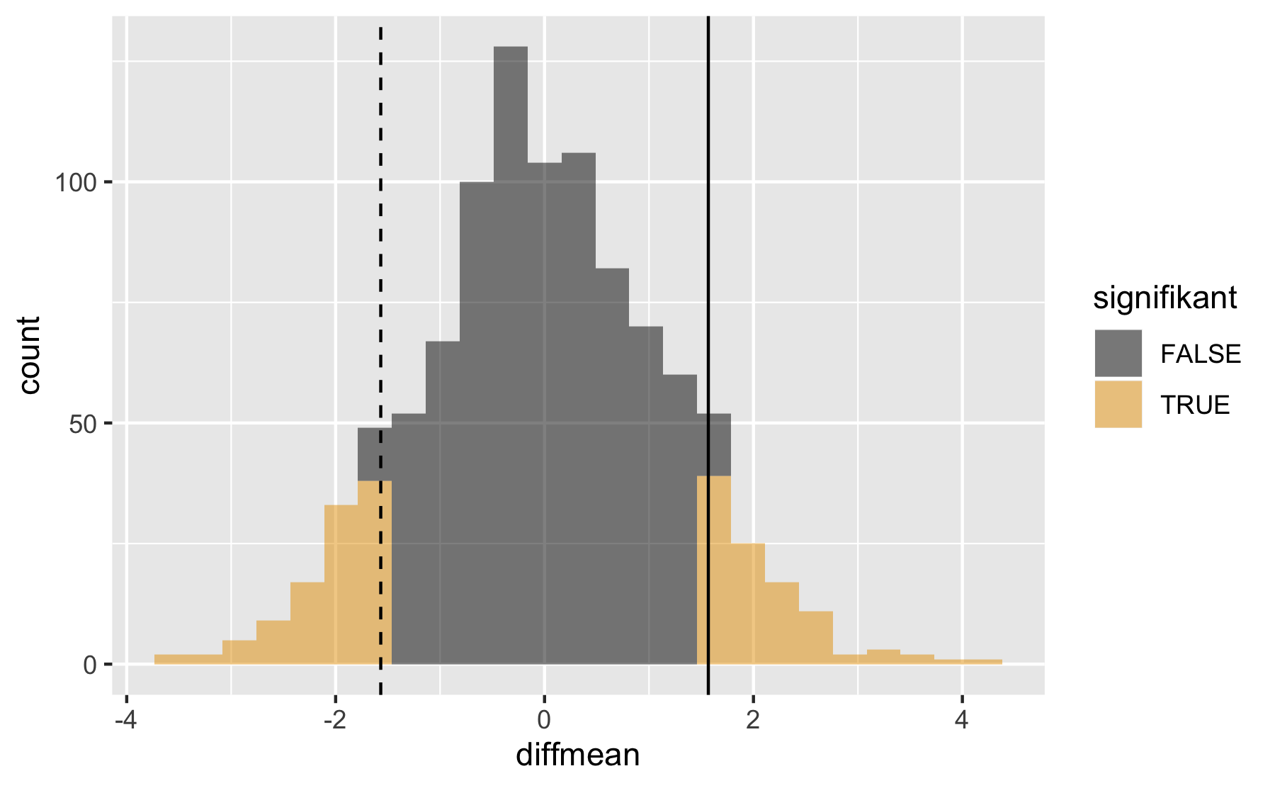
Verteilungsbasiert vs. simulationsbasiert
Sinnbild: Bootstrap
Sinnbild: Zusammenhang zweier Variablen (Permutationstest)
Sinnbild: Test auf bestimmten Wert einer Variablen