1 Load packages
library(tidyverse)  # data wrangling
library(see)  # okabeito_colors
2 Data
data("mariokart", package = "openintro")3 Unadjusted labels
mario_quantile <-
mariokart %>%
  filter(total_pr < 100) %>%
  summarise(q25 = quantile(total_pr, .25),
            q50 = quantile(total_pr, .50),
            q75 = quantile(total_pr, .75))

mario_quantile <-
  mariokart %>%
  filter(total_pr < 100) %>%
  reframe(qs = quantile(total_pr, c(.25, .5, .75)))

mariokart %>%
  filter(total_pr < 100) %>%
  ggplot(aes(x = total_pr)) +
  geom_histogram() +
  geom_vline(xintercept = mario_quantile$qs) +
  annotate("label", x =  mario_quantile$qs, y = 0, label =  mario_quantile$qs) +
annotate("label", x = mario_quantile$qs, y = Inf, label = c("Q1", "Median", "Q3")) 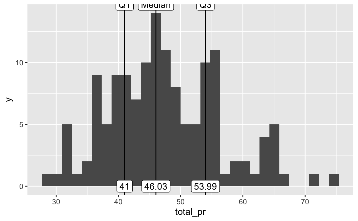
4 Adjusted labels manually
vjust = 2 does the trick:
mario_quantile <-
mariokart %>%
  filter(total_pr < 100) %>%
  summarise(q25 = quantile(total_pr, .25),
            q50 = quantile(total_pr, .50),
            q75 = quantile(total_pr, .75))

mario_quantile <-
  mariokart %>%
  filter(total_pr < 100) %>%
  reframe(qs = quantile(total_pr, c(.25, .5, .75)))

mariokart %>%
  filter(total_pr < 100) %>%
  ggplot(aes(x = total_pr)) +
  geom_histogram() +
  geom_vline(xintercept = mario_quantile$qs) +
  annotate("label", x =  mario_quantile$qs, y = 0, label =  mario_quantile$qs) +
annotate("label", x = mario_quantile$qs, y = Inf, label = c("Q1", "Median", "Q3"), vjust = 2) 
5 Adjust labels automatically
Using vjust = "top" (or “bottom”) does the trick in an automatic, comfortable way.
mariokart %>%
  filter(total_pr < 100) %>%
  ggplot(aes(x = total_pr)) +
  geom_histogram() +
  geom_vline(xintercept = mario_quantile$qs) +
  annotate("label", x =  mario_quantile$qs, y = 0, label =  mario_quantile$qs, vjust = "bottom") +
annotate("label", x = mario_quantile$qs, y = Inf, label = c("Q1", "Median", "Q3"), vjust = "top") 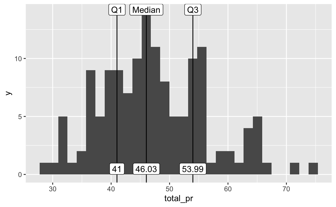
Similarly, one case use hjust = "left" for horizontal alignment.
6 Expanding the limits
Let’s consider a second example, where it helped to expand the limits of the coordinates.
In this example, we use Weather data from the German DWD i.e., Deutschen Wetterdienst, DWD .
After some data wrangling, which will not discussed here, there’s a nice data set waiting for further scrutiny.
wetter_path <- "https://raw.githubusercontent.com/sebastiansauer/Lehre/main/data/wetter-dwd/precip_temp_DWD.csv"
wetter <- read.csv(wetter_path)
Some data preparation:
wetter <-
  wetter %>%
  mutate(after_1950 = year > 1950) %>%
  filter(region != "Deutschland")  # ohne Daten für Gesamt-Deutschland
Here’s a linear model for our weather data:
lm_wetter_region <- lm(temp ~ region, data = wetter)wetter_summ <-
wetter %>%
group_by(region) %>%
summarise(temp = mean(temp)) %>%
mutate(id = 0:15) %>%
ungroup() %>%
mutate(grandmean = mean(temp),
delta = temp - grandmean)
wetter_summ %>%
ggplot(aes(y = region, x = temp)) +
theme_minimal() +
geom_label(aes(label = paste0("b", id),
x = grandmean + delta),
vjust = 1,
size = 2,
color = okabeito_colors()[1]) +
geom_vline(xintercept = coef(lm_wetter_region)[1], linetype = "dashed", color = okabeito_colors()[2]) +
#coord_cartesian(xlim = c(7, 10), ylim = c(0, 16)) +
annotate("label",
y = 1,
x = coef(lm_wetter_region)[1],
vjust = 1,
label = paste0("b0"),
#size = 6,
color = okabeito_colors()[2]) +
annotate("point",
y = 1,
x = coef(lm_wetter_region)[1],
color = okabeito_colors()[2],
#vjust = 1,
size = 4) +
geom_segment(aes(yend = region, xend = temp),
x = coef(lm_wetter_region)[1],
color = okabeito_colors()[1]) +
geom_point() +
labs(y = "",
x = "Temperatur")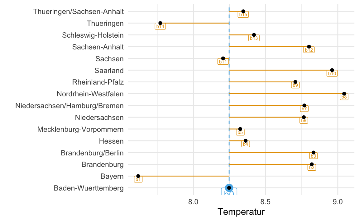
Behold the label right at the bottom of the diagram, “b0”. It is not displayed properly.
One way to get it back into the picture is bay extending the limits of the y-axis:
wetter_summ %>%
  ggplot(aes(y = region, x = temp)) +
  theme_minimal() +
  geom_label(aes(label = paste0("b", id),
                 x = grandmean + delta),
             vjust = 1,
             size = 2,
             color = okabeito_colors()[1]) +
  geom_vline(xintercept = coef(lm_wetter_region)[1], linetype = "dashed", color = okabeito_colors()[2]) +

 coord_cartesian(xlim = c(7, 10), ylim = c(0, 16))  +  # back in the game!

  annotate("label",
           y = 1,
           x = coef(lm_wetter_region)[1],
           vjust = 1,
           label = paste0("b0"),
           #size = 6,
           color = okabeito_colors()[2]) +
  annotate("point",
           y = 1,
           x = coef(lm_wetter_region)[1],
           color = okabeito_colors()[2],
           #vjust = 1,
           size = 4) +
  geom_segment(aes(yend = region, xend = temp),
               x = coef(lm_wetter_region)[1],
               color = okabeito_colors()[1])  +
    geom_point() +
  labs(y = "",
       x = "Temperatur")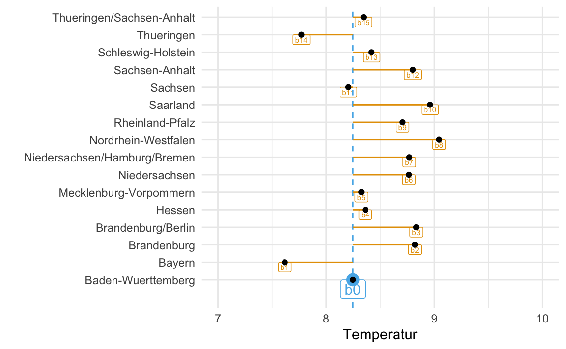
7 Duckdive the problem: tinyfy the label
It may feel like cheating, but, hey, problem solved: just decrease the size of the label.
wetter_summ %>%
  ggplot(aes(y = region, x = temp)) +
  theme_minimal() +
  geom_point() +
  annotate("point",
           y = 1,
           x = coef(lm_wetter_region)[1],
           color = okabeito_colors()[2],
           size = 4,
           alpha = .5) +
  geom_label(aes(label = paste0("b", id),
                 x = grandmean + delta),
             vjust = 1,
             size = 2,
             color = okabeito_colors()[1]) +
  geom_vline(xintercept = coef(lm_wetter_region)[1],
             linetype = "dashed", color = okabeito_colors()[2]) +

  #coord_cartesian(xlim = c(7, 10), ylim = c(0, 16))  +

  annotate("label",
           y = 1,
           x = coef(lm_wetter_region)[1],
           vjust = 1,
           label = paste0("b0"),
           size = 2,
           color = okabeito_colors()[2]) +

  geom_segment(aes(yend = region, xend = temp),
               x = coef(lm_wetter_region)[1],
               color = okabeito_colors()[1])  +
  labs(y = "",
       x = "Temperatur")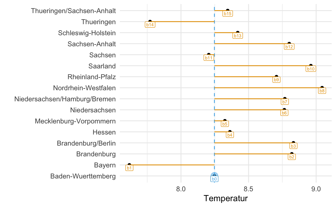
8 Reproducibility
#> ─ Session info ───────────────────────────────────────────────────────────────────────────────────────────────────────
#>  setting  value
#>  version  R version 4.2.1 (2022-06-23)
#>  os       macOS Big Sur ... 10.16
#>  system   x86_64, darwin17.0
#>  ui       X11
#>  language (EN)
#>  collate  en_US.UTF-8
#>  ctype    en_US.UTF-8
#>  tz       Europe/Berlin
#>  date     2024-02-25
#>  pandoc   3.1.12.1 @ /usr/local/bin/ (via rmarkdown)
#>
#> ─ Packages ───────────────────────────────────────────────────────────────────────────────────────────────────────────
#>  package     * version date (UTC) lib source
#>  blogdown      1.18    2023-06-19 [1] CRAN (R 4.2.0)
#>  bookdown      0.36    2023-10-16 [1] CRAN (R 4.2.0)
#>  bslib         0.6.1   2023-11-28 [1] CRAN (R 4.2.0)
#>  cachem        1.0.8   2023-05-01 [1] CRAN (R 4.2.0)
#>  callr         3.7.3   2022-11-02 [1] CRAN (R 4.2.0)
#>  cli           3.6.2   2023-12-11 [1] CRAN (R 4.2.0)
#>  codetools     0.2-19  2023-02-01 [1] CRAN (R 4.2.0)
#>  colorspace    2.1-0   2023-01-23 [1] CRAN (R 4.2.0)
#>  crayon        1.5.2   2022-09-29 [1] CRAN (R 4.2.1)
#>  devtools      2.4.5   2022-10-11 [1] CRAN (R 4.2.1)
#>  digest        0.6.33  2023-07-07 [1] CRAN (R 4.2.0)
#>  dplyr       * 1.1.4   2023-11-17 [1] CRAN (R 4.2.0)
#>  ellipsis      0.3.2   2021-04-29 [1] CRAN (R 4.2.0)
#>  evaluate      0.23    2023-11-01 [1] CRAN (R 4.2.0)
#>  fansi         1.0.6   2023-12-08 [1] CRAN (R 4.2.0)
#>  farver        2.1.1   2022-07-06 [1] CRAN (R 4.2.0)
#>  fastmap       1.1.1   2023-02-24 [1] CRAN (R 4.2.0)
#>  forcats     * 1.0.0   2023-01-29 [1] CRAN (R 4.2.0)
#>  fs            1.6.3   2023-07-20 [1] CRAN (R 4.2.0)
#>  generics      0.1.3   2022-07-05 [1] CRAN (R 4.2.0)
#>  ggplot2     * 3.5.0   2024-02-23 [1] CRAN (R 4.2.1)
#>  glue          1.6.2   2022-02-24 [1] CRAN (R 4.2.0)
#>  gtable        0.3.4   2023-08-21 [1] CRAN (R 4.2.0)
#>  highr         0.10    2022-12-22 [1] CRAN (R 4.2.0)
#>  hms           1.1.3   2023-03-21 [1] CRAN (R 4.2.0)
#>  htmltools     0.5.7   2023-11-03 [1] CRAN (R 4.2.0)
#>  htmlwidgets   1.6.2   2023-03-17 [1] CRAN (R 4.2.0)
#>  httpuv        1.6.11  2023-05-11 [1] CRAN (R 4.2.0)
#>  jquerylib     0.1.4   2021-04-26 [1] CRAN (R 4.2.0)
#>  jsonlite      1.8.8   2023-12-04 [1] CRAN (R 4.2.0)
#>  knitr         1.45    2023-10-30 [1] CRAN (R 4.2.1)
#>  labeling      0.4.3   2023-08-29 [1] CRAN (R 4.2.0)
#>  later         1.3.1   2023-05-02 [1] CRAN (R 4.2.0)
#>  lifecycle     1.0.4   2023-11-07 [1] CRAN (R 4.2.1)
#>  lubridate   * 1.9.3   2023-09-27 [1] CRAN (R 4.2.0)
#>  magrittr      2.0.3   2022-03-30 [1] CRAN (R 4.2.0)
#>  memoise       2.0.1   2021-11-26 [1] CRAN (R 4.2.0)
#>  mime          0.12    2021-09-28 [1] CRAN (R 4.2.0)
#>  miniUI        0.1.1.1 2018-05-18 [1] CRAN (R 4.2.0)
#>  munsell       0.5.0   2018-06-12 [1] CRAN (R 4.2.0)
#>  pillar        1.9.0   2023-03-22 [1] CRAN (R 4.2.0)
#>  pkgbuild      1.4.0   2022-11-27 [1] CRAN (R 4.2.0)
#>  pkgconfig     2.0.3   2019-09-22 [1] CRAN (R 4.2.0)
#>  pkgload       1.3.2.1 2023-07-08 [1] CRAN (R 4.2.0)
#>  prettyunits   1.1.1   2020-01-24 [1] CRAN (R 4.2.0)
#>  processx      3.8.2   2023-06-30 [1] CRAN (R 4.2.0)
#>  profvis       0.3.8   2023-05-02 [1] CRAN (R 4.2.0)
#>  promises      1.2.1   2023-08-10 [1] CRAN (R 4.2.0)
#>  ps            1.7.5   2023-04-18 [1] CRAN (R 4.2.0)
#>  purrr       * 1.0.2   2023-08-10 [1] CRAN (R 4.2.0)
#>  R6            2.5.1   2021-08-19 [1] CRAN (R 4.2.0)
#>  Rcpp          1.0.11  2023-07-06 [1] CRAN (R 4.2.0)
#>  readr       * 2.1.4   2023-02-10 [1] CRAN (R 4.2.0)
#>  remotes       2.4.2.1 2023-07-18 [1] CRAN (R 4.2.0)
#>  rlang         1.1.2   2023-11-04 [1] CRAN (R 4.2.0)
#>  rmarkdown     2.25    2023-09-18 [1] CRAN (R 4.2.0)
#>  rstudioapi    0.15.0  2023-07-07 [1] CRAN (R 4.2.0)
#>  sass          0.4.8   2023-12-06 [1] CRAN (R 4.2.0)
#>  scales        1.3.0   2023-11-28 [1] CRAN (R 4.2.0)
#>  sessioninfo   1.2.2   2021-12-06 [1] CRAN (R 4.2.0)
#>  shiny         1.8.0   2023-11-17 [1] CRAN (R 4.2.1)
#>  stringi       1.8.3   2023-12-11 [1] CRAN (R 4.2.0)
#>  stringr     * 1.5.1   2023-11-14 [1] CRAN (R 4.2.1)
#>  tibble      * 3.2.1   2023-03-20 [1] CRAN (R 4.2.0)
#>  tidyr       * 1.3.0   2023-01-24 [1] CRAN (R 4.2.0)
#>  tidyselect    1.2.0   2022-10-10 [1] CRAN (R 4.2.0)
#>  tidyverse   * 2.0.0   2023-02-22 [1] CRAN (R 4.2.0)
#>  timechange    0.2.0   2023-01-11 [1] CRAN (R 4.2.0)
#>  tzdb          0.4.0   2023-05-12 [1] CRAN (R 4.2.0)
#>  urlchecker    1.0.1   2021-11-30 [1] CRAN (R 4.2.0)
#>  usethis       2.2.2   2023-07-06 [1] CRAN (R 4.2.0)
#>  utf8          1.2.4   2023-10-22 [1] CRAN (R 4.2.0)
#>  vctrs         0.6.5   2023-12-01 [1] CRAN (R 4.2.0)
#>  withr         3.0.0   2024-01-16 [1] CRAN (R 4.2.1)
#>  xfun          0.41    2023-11-01 [1] CRAN (R 4.2.0)
#>  xtable        1.8-4   2019-04-21 [1] CRAN (R 4.2.0)
#>  yaml          2.3.8   2023-12-11 [1] CRAN (R 4.2.0)
#>
#>  [1] /Users/sebastiansaueruser/Rlibs
#>  [2] /Library/Frameworks/R.framework/Versions/4.2/Resources/library
#>
#> ──────────────────────────────────────────────────────────────────────────────────────────────────────────────────────