1 Load packages
library(tidyverse)  # data wrangling
library(easystats)
library(ggplot2); theme_set(theme_minimal())  # ggplot theme
2 Motivation
Let’s explore the change over time in German weather. We are not pretending doing real meteorology here; rather, we are playing around a bit. At the very least, we’ll do over own analyses, so we know what’s going in. Data stems from Deutscher Wetter Diensts, DWD.
3 Load data
The DWD data has been prepared from fast consumption as laid out in this post.
As a result, the data have been made available in this repo.
d_path <- "https://raw.githubusercontent.com/sebastiansauer/datasets/main/csv/precip_temp_DWD.csv"

d <- read_csv(d_path)
glimpse(d)
#> Rows: 28,866
#> Columns: 5
#> $ year <dbl> 1881, 1881, 1881, 1881, 1881, 1881, 1881, 1881, 1881, 1881, 188…
#> $ month <dbl> 1, 1, 1, 1, 1, 1, 1, 1, 1, 1, 1, 1, 1, 1, 1, 1, 1, 1, 1, 1, 1, …
#> $ region <chr> "Brandenburg/Berlin", "Brandenburg", "Baden-Wuerttemberg", "Bay…
#> $ precip <dbl> 20.4, 20.3, 36.2, 22.5, 33.2, 16.8, 35.1, 34.9, 40.6, 39.3, 21.…
#> $ temp <dbl> -5.54, -5.56, -4.89, -6.51, -5.68, -5.07, -4.55, -4.55, -4.21, …4 Main temperature trajectory over time
4.1 Visualization
d_grouped <-
  d %>%
  group_by(region, year) %>%
  summarise(temp_avg = mean(temp))

d_grouped %>%
  ggplot(aes(x = year, y = temp_avg, group = region)) +
  geom_line(color = "grey60") +
  labs(title = "Temperature change over time in Germany",
       caption = "Data Source: DWD",
       subtitle = "One grey line depicts one Bundesland") +
geom_smooth(method = "lm", group = 1) 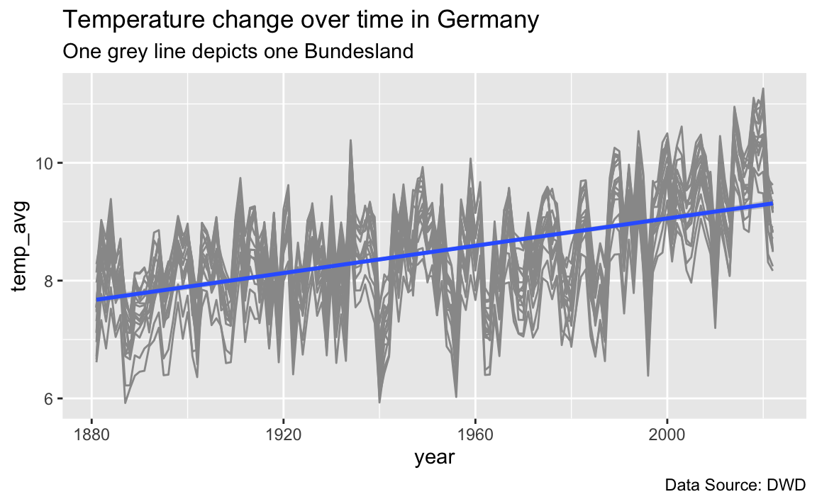
Temperature is on the rise, it appears.
4.2 Linear model
m1 <- lm(temp_avg ~ year, data = d_grouped)
print_html(model_parameters(m1))| Model Summary | |||||
|---|---|---|---|---|---|
| Parameter | Coefficient | SE | 95% CI | t(2412) | p |
| (Intercept) | -14.14 | 0.77 | (-15.64, -12.63) | -18.45 | < .001 |
| year | 0.01 | 3.93e-04 | (0.01, 0.01) | 29.54 | < .001 |
This amounts to approx. 0.1 degrees Celcius per Dekade on average.
plot(parameters(m1), show_intercept = TRUE)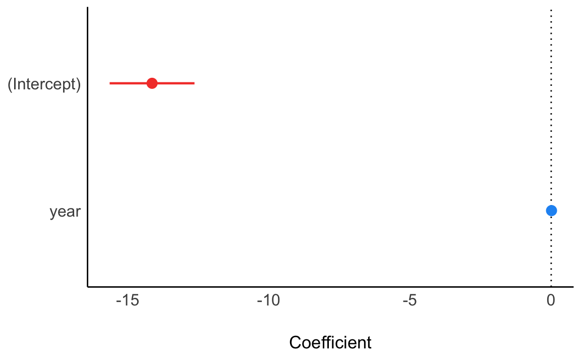
5 Temperature change per month
5.1 Vis 1: Change per Month for whole of Germany
d_grouped2 <-
d %>%
group_by(region, year, month) %>%
summarise(temp_avg = mean(temp))
d_grouped2 %>%
ggplot(aes(x = year, y = temp_avg, group = region)) +
geom_line(color = "grey60") +
labs(title = "Temperature change over time per month") +
facet_wrap(~ month, ncol = 3) +
geom_smooth(method = "lm", group = 1)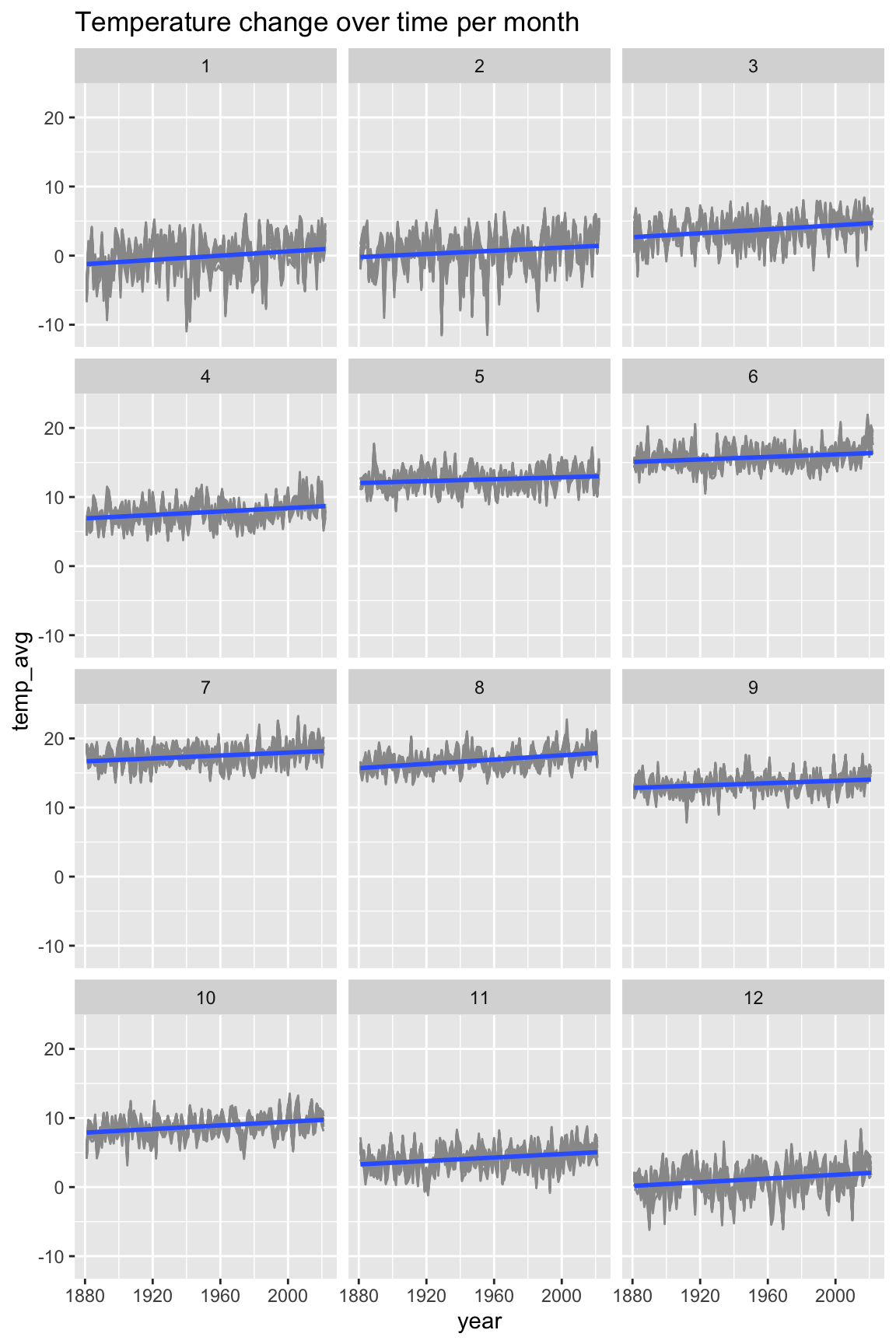 It looks like that for each month, temperature is on the rise.
I don’t think it is very important to check this trend for each Bundesland. However, it may well be that this trend is more pronounced for some Bundesländer as opposed to others.
5.2 Linear model
m2 <- lm(temp_avg ~ as.factor(month) + year, data = d_grouped2)
print_html(model_parameters(m2))| Model Summary | |||||
|---|---|---|---|---|---|
| Parameter | Coefficient | SE | 95% CI | t(28853) | p |
| (Intercept) | -23.41 | 0.54 | (-24.46, -22.35) | -43.56 | < .001 |
| month (2) | 0.74 | 0.05 | (0.63, 0.85) | 13.49 | < .001 |
| month (3) | 3.83 | 0.05 | (3.72, 3.93) | 69.75 | < .001 |
| month (4) | 7.93 | 0.05 | (7.83, 8.04) | 144.62 | < .001 |
| month (5) | 12.65 | 0.05 | (12.55, 12.76) | 230.64 | < .001 |
| month (6) | 15.86 | 0.05 | (15.75, 15.97) | 289.06 | < .001 |
| month (7) | 17.57 | 0.05 | (17.46, 17.68) | 319.71 | < .001 |
| month (8) | 16.94 | 0.05 | (16.83, 17.05) | 308.19 | < .001 |
| month (9) | 13.59 | 0.05 | (13.48, 13.69) | 247.21 | < .001 |
| month (10) | 8.95 | 0.05 | (8.84, 9.06) | 162.90 | < .001 |
| month (11) | 4.31 | 0.05 | (4.20, 4.42) | 78.40 | < .001 |
| month (12) | 1.26 | 0.05 | (1.16, 1.37) | 23.00 | < .001 |
| year | 0.01 | 2.75e-04 | (0.01, 0.01) | 43.42 | < .001 |
plot(parameters(m2), show_intercept = TRUE)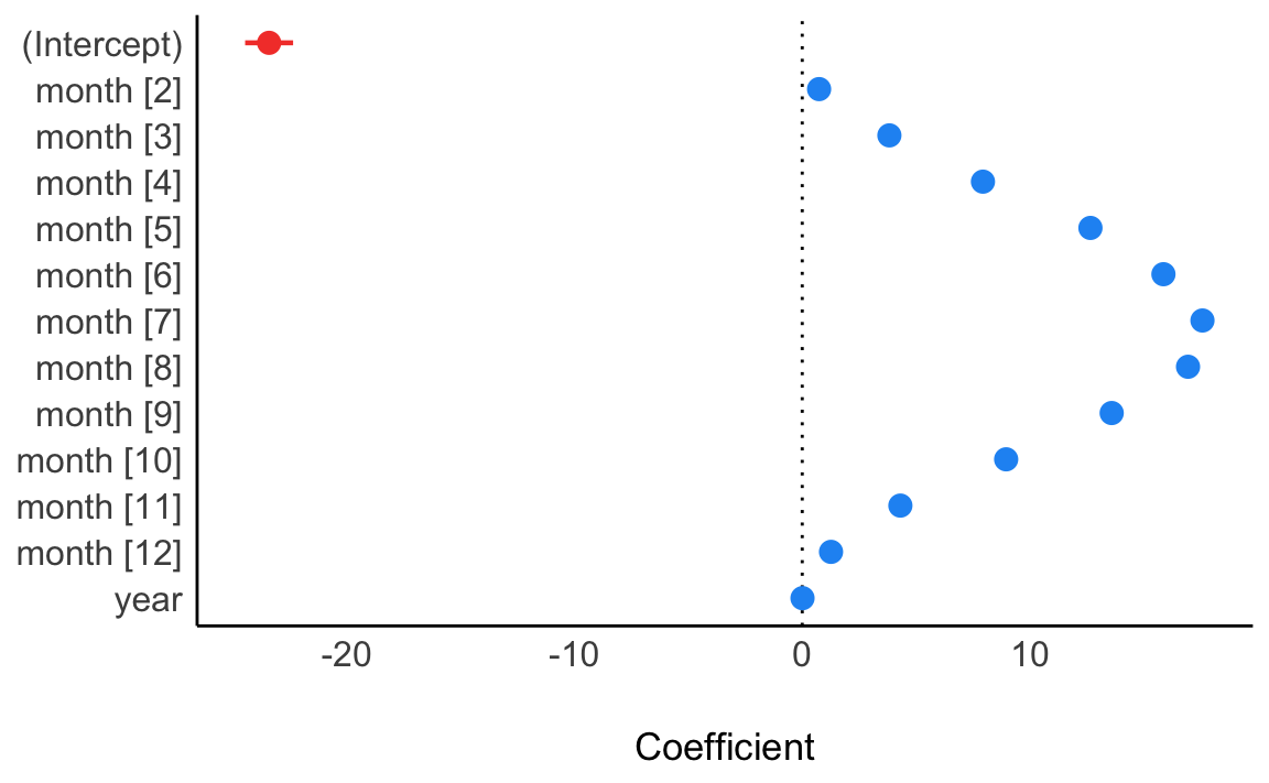
Here we see the effect of the month, with the Month of July being the warmest, which makes sense. Note that the intercept is not interpretable here as it shows the temperature in year 0, which is a bit far away.
For comparison, let’s just see the avarage temperatures per month:
m3 <- lm(temp_avg ~ as.factor(month), data = d_grouped2)
print_html(model_parameters(m3))| Model Summary | |||||
|---|---|---|---|---|---|
| Parameter | Coefficient | SE | 95% CI | t(28854) | p |
| (Intercept) | -0.13 | 0.04 | (-0.21, -0.06) | -3.36 | < .001 |
| month (2) | 0.74 | 0.06 | (0.63, 0.85) | 13.07 | < .001 |
| month (3) | 3.83 | 0.06 | (3.72, 3.94) | 67.57 | < .001 |
| month (4) | 7.93 | 0.06 | (7.82, 8.04) | 140.12 | < .001 |
| month (5) | 12.65 | 0.06 | (12.54, 12.76) | 223.46 | < .001 |
| month (6) | 15.86 | 0.06 | (15.75, 15.97) | 280.06 | < .001 |
| month (7) | 17.57 | 0.06 | (17.45, 17.68) | 309.65 | < .001 |
| month (8) | 16.93 | 0.06 | (16.82, 17.04) | 298.49 | < .001 |
| month (9) | 13.58 | 0.06 | (13.47, 13.69) | 239.40 | < .001 |
| month (10) | 8.95 | 0.06 | (8.84, 9.06) | 157.72 | < .001 |
| month (11) | 4.30 | 0.06 | (4.19, 4.41) | 75.86 | < .001 |
| month (12) | 1.26 | 0.06 | (1.15, 1.37) | 22.18 | < .001 |
Note that these are the averages across all the years in the data set.
plot(parameters(m3), show_intercept = TRUE)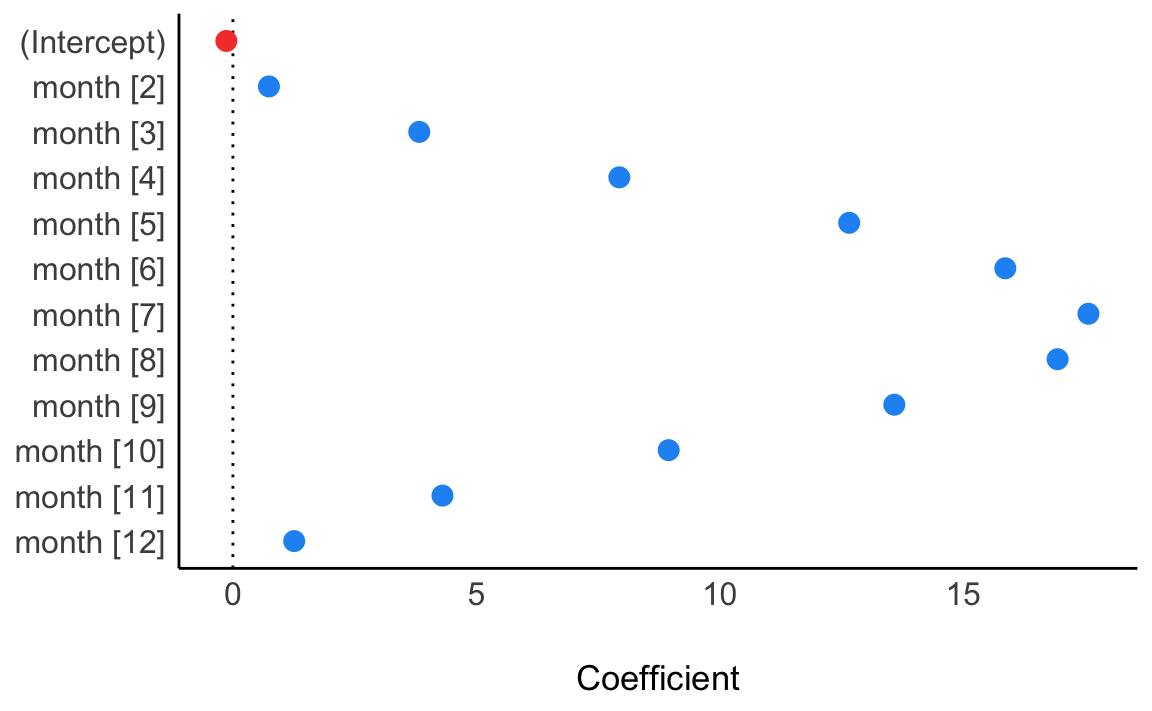
5.3 Vis 2: Trend by Bundesland
d_grouped2a <-
  d %>%
  group_by(region, year) %>%
  summarise(temp_avg = mean(temp))

d_grouped2a %>%
  ggplot(aes(x = year, y = temp_avg)) +
  geom_line(color = "grey60") +
  labs(title = "Temperature change over time per Bundesland") +
  facet_wrap(~ region, ncol = 3) +
  geom_smooth(method = "lm")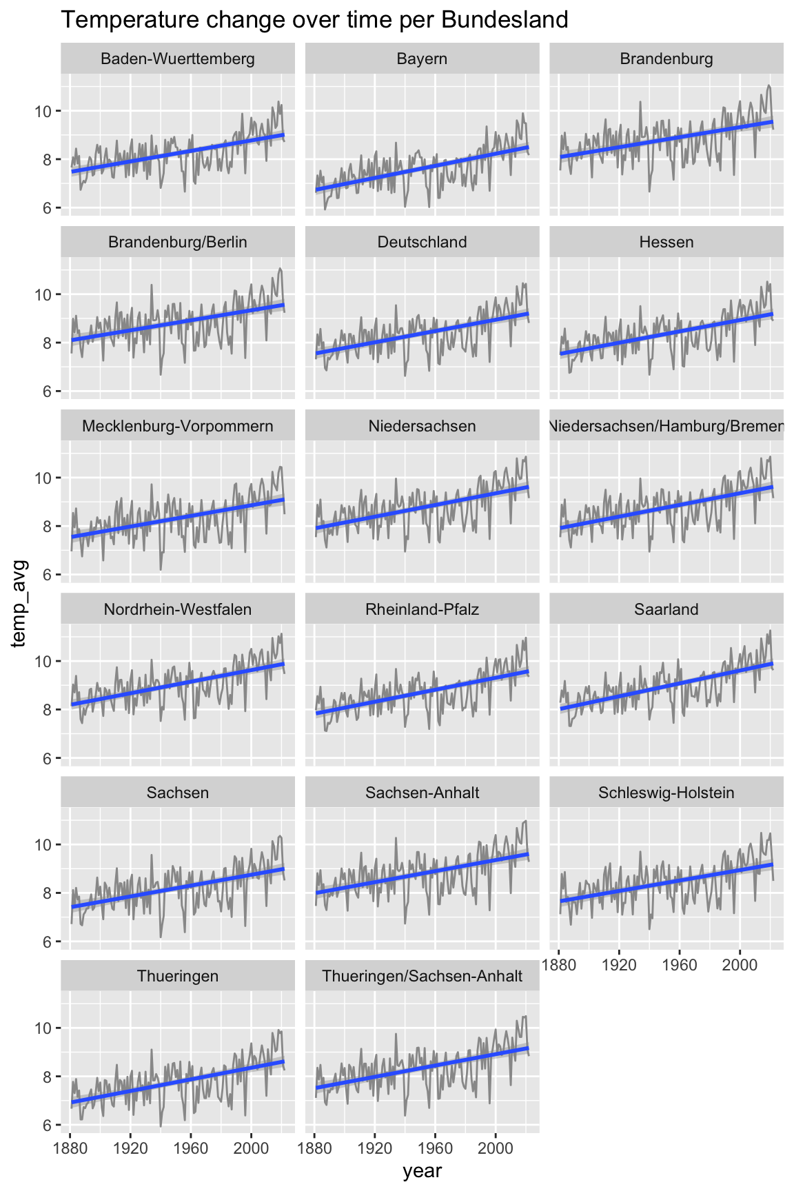
m4 <- lm(temp ~ region + year, data = d)
print_html(parameters(m4))| Model Summary | |||||
|---|---|---|---|---|---|
| Parameter | Coefficient | SE | 95% CI | t(28848) | p |
| (Intercept) | -14.49 | 1.85 | (-18.13, -10.86) | -7.82 | < .001 |
| region (Bayern) | -0.63 | 0.23 | (-1.07, -0.19) | -2.79 | 0.005 |
| region (Brandenburg) | 0.57 | 0.23 | (0.13, 1.01) | 2.54 | 0.011 |
| region (Brandenburg/Berlin) | 0.58 | 0.23 | (0.14, 1.03) | 2.59 | 0.009 |
| region (Deutschland) | 0.13 | 0.23 | (-0.31, 0.57) | 0.58 | 0.563 |
| region (Hessen) | 0.11 | 0.23 | (-0.33, 0.56) | 0.51 | 0.611 |
| region (Mecklenburg-Vorpommern) | 0.08 | 0.23 | (-0.36, 0.52) | 0.34 | 0.732 |
| region (Niedersachsen) | 0.52 | 0.23 | (0.08, 0.96) | 2.30 | 0.022 |
| region (Niedersachsen/Hamburg/Bremen) | 0.52 | 0.23 | (0.08, 0.96) | 2.31 | 0.021 |
| region (Nordrhein-Westfalen) | 0.80 | 0.23 | (0.36, 1.24) | 3.54 | < .001 |
| region (Rheinland-Pfalz) | 0.46 | 0.23 | (0.02, 0.90) | 2.04 | 0.042 |
| region (Saarland) | 0.71 | 0.23 | (0.27, 1.16) | 3.17 | 0.002 |
| region (Sachsen) | -0.04 | 0.23 | (-0.48, 0.40) | -0.19 | 0.853 |
| region (Sachsen-Anhalt) | 0.55 | 0.23 | (0.11, 1.00) | 2.46 | 0.014 |
| region (Schleswig-Holstein) | 0.17 | 0.23 | (-0.27, 0.61) | 0.76 | 0.445 |
| region (Thueringen) | -0.48 | 0.23 | (-0.92, -0.03) | -2.11 | 0.035 |
| region (Thueringen/Sachsen-Anhalt) | 0.10 | 0.23 | (-0.34, 0.54) | 0.44 | 0.663 |
| year | 0.01 | 9.46e-04 | (9.80e-03, 0.01) | 12.32 | < .001 |
The point estimate indicates that Saarland gained most in terms of temperature; however, the differences are not clear cut between the Bundesländer, so no strong conclusion can be drawn.
6 Change per decade
d2 <-
  d %>%
  mutate(decade = trunc(year  / 10))

head(d2)
#> # A tibble: 6 × 6
#>    year month region                 precip  temp decade
#>   <dbl> <dbl> <chr>                   <dbl> <dbl>  <dbl>
#> 1  1881     1 Brandenburg/Berlin       20.4 -5.54    188
#> 2  1881     1 Brandenburg              20.3 -5.56    188
#> 3  1881     1 Baden-Wuerttemberg       36.2 -4.89    188
#> 4  1881     1 Bayern                   22.5 -6.51    188
#> 5  1881     1 Hessen                   33.2 -5.68    188
#> 6  1881     1 Mecklenburg-Vorpommern   16.8 -5.07    188
d_grouped3 <-
d2 %>%
group_by(region, decade) %>%
summarise(temp_avg = mean(temp)) %>%
mutate(temp_dec_before = lag(temp_avg)) %>%
mutate(temp_change_decade = temp_avg - temp_dec_before)
d_grouped3 %>%
head()
#> # A tibble: 6 × 5
#> # Groups: region [1]
#> region decade temp_avg temp_dec_before temp_change_decade
#> <chr> <dbl> <dbl> <dbl> <dbl>
#> 1 Baden-Wuerttemberg 188 7.63 NA NA
#> 2 Baden-Wuerttemberg 189 7.79 7.63 0.156
#> 3 Baden-Wuerttemberg 190 7.82 7.79 0.0274
#> 4 Baden-Wuerttemberg 191 7.98 7.82 0.166
#> 5 Baden-Wuerttemberg 192 8.09 7.98 0.110
#> 6 Baden-Wuerttemberg 193 8.08 8.09 -0.01556.1 Vis 1
d_grouped3 %>%
  ggplot(aes(x = decade, y = temp_avg)) +
  geom_point(color = "grey60") +
  labs(title = "Temperature change over decades in Germany",
       caption = "Data Source: DWD",
       subtitle = "One grey dot depicts one Bundesland",
       y = "Temperature in °C") +
  stat_summary(geom = "line", fun = mean) +
  scale_x_continuous(breaks = 188:202)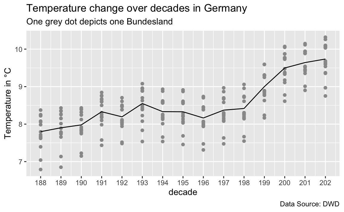
Again, we see that temperature is on the rise.
6.2 Vis 2: Temperature change per decade
d_grouped3 %>%
  ggplot(aes(x = decade, y = temp_change_decade)) +
  geom_point(color = "grey60") +
  labs(title = "Temperature change over decades in Germany",
       caption = "Data Source: DWD",
       subtitle = "One grey dot depicts one Bundesland") +
  stat_summary(geom = "line", fun = mean) +
  scale_x_continuous(breaks = 188:202)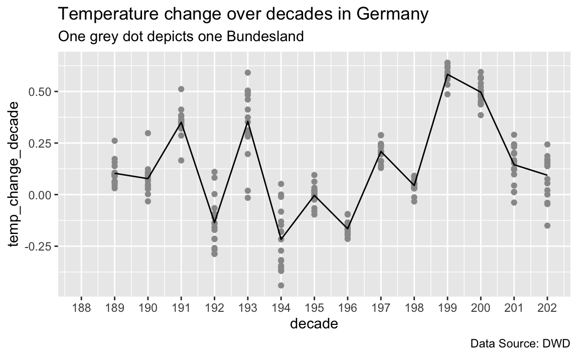
For any to given subsequent decades, we see that the the average temperature of the decase has risen. This trend is most pronounced in the 1990 and 2000 decades; but it is positive (hotter) for any data point in this graph AFTER 1960.
7 Change in variability
d_grouped4 <-
  d2 %>%
  group_by(region, decade) %>%
  summarise(temp_sd = sd(temp)) %>%
  mutate(temp_sd_dec_before = lag(temp_sd)) %>%
  mutate(temp_sd_change_decade = temp_sd - temp_sd_dec_before)

d_grouped4 %>%
  head()
#> # A tibble: 6 × 5
#> # Groups:   region [1]
#>   region             decade temp_sd temp_sd_dec_before temp_sd_change_decade
#>   <chr>               <dbl>   <dbl>              <dbl>                 <dbl>
#> 1 Baden-Wuerttemberg    188    6.80              NA                  NA
#> 2 Baden-Wuerttemberg    189    6.90               6.80                0.107
#> 3 Baden-Wuerttemberg    190    6.70               6.90               -0.208
#> 4 Baden-Wuerttemberg    191    6.21               6.70               -0.484
#> 5 Baden-Wuerttemberg    192    6.51               6.21                0.299
#> 6 Baden-Wuerttemberg    193    6.57               6.51                0.0571
7.1 Vis
d_grouped4 %>%
  ggplot(aes(x = decade, y = temp_sd)) +
  geom_point(color = "grey60") +
  labs(title = "Temperature *variability* change over decades in Germany",
       caption = "Data Source: DWD",
       subtitle = "One grey dot depicts one Bundesland") +
  stat_summary(geom = "line", fun = mean) +
  scale_x_continuous(breaks = 188:202)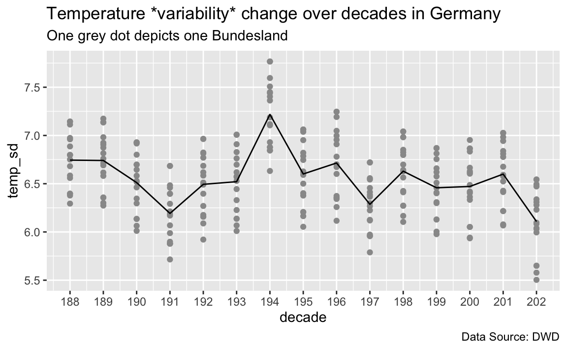
Apart from the 1940, there’s no apparent change in variability (SD) per decade.
8 Debrief
This post is NOT real meteorology science! Rather, it is some exploratory appraoching to a highly sophisticated field of research. Certainly, the state of art is not reflected in this post. The (aspired) benefit of this post is to bring the data-savy layman closer to weather data in an attempt not to have to (completely) rely on third persons.
9 Reproducibility
#> ─ Session info ───────────────────────────────────────────────────────────────────────────────────────────────────────
#>  setting  value
#>  version  R version 4.2.0 (2022-04-22)
#>  os       macOS Big Sur/Monterey 10.16
#>  system   x86_64, darwin17.0
#>  ui       X11
#>  language (EN)
#>  collate  en_US.UTF-8
#>  ctype    en_US.UTF-8
#>  tz       Europe/Berlin
#>  date     2022-07-24
#>  pandoc   2.18 @ /usr/local/bin/ (via rmarkdown)
#>
#> ─ Packages ───────────────────────────────────────────────────────────────────────────────────────────────────────────
#>  package       * version date (UTC) lib source
#>  assertthat      0.2.1   2019-03-21 [1] CRAN (R 4.2.0)
#>  backports       1.4.1   2021-12-13 [1] CRAN (R 4.2.0)
#>  blogdown        1.10    2022-05-10 [1] CRAN (R 4.2.0)
#>  bookdown        0.27    2022-06-14 [1] CRAN (R 4.2.0)
#>  broom           1.0.0   2022-07-01 [1] CRAN (R 4.2.0)
#>  bslib           0.4.0   2022-07-16 [1] CRAN (R 4.2.0)
#>  cachem          1.0.6   2021-08-19 [1] CRAN (R 4.2.0)
#>  callr           3.7.1   2022-07-13 [1] CRAN (R 4.2.0)
#>  cellranger      1.1.0   2016-07-27 [1] CRAN (R 4.2.0)
#>  cli             3.3.0   2022-04-25 [1] CRAN (R 4.2.0)
#>  codetools       0.2-18  2020-11-04 [2] CRAN (R 4.2.0)
#>  colorout      * 1.2-2   2022-06-13 [1] local
#>  colorspace      2.0-3   2022-02-21 [1] CRAN (R 4.2.0)
#>  crayon          1.5.1   2022-03-26 [1] CRAN (R 4.2.0)
#>  DBI             1.1.3   2022-06-18 [1] CRAN (R 4.2.0)
#>  dbplyr          2.2.1   2022-06-27 [1] CRAN (R 4.2.0)
#>  devtools        2.4.4   2022-07-20 [1] CRAN (R 4.2.0)
#>  digest          0.6.29  2021-12-01 [1] CRAN (R 4.2.0)
#>  dplyr         * 1.0.9   2022-04-28 [1] CRAN (R 4.2.0)
#>  ellipsis        0.3.2   2021-04-29 [1] CRAN (R 4.2.0)
#>  evaluate        0.15    2022-02-18 [1] CRAN (R 4.2.0)
#>  fansi           1.0.3   2022-03-24 [1] CRAN (R 4.2.0)
#>  fastmap         1.1.0   2021-01-25 [1] CRAN (R 4.2.0)
#>  forcats       * 0.5.1   2021-01-27 [1] CRAN (R 4.2.0)
#>  fs              1.5.2   2021-12-08 [1] CRAN (R 4.2.0)
#>  gargle          1.2.0   2021-07-02 [1] CRAN (R 4.2.0)
#>  generics        0.1.3   2022-07-05 [1] CRAN (R 4.2.0)
#>  ggplot2       * 3.3.6   2022-05-03 [1] CRAN (R 4.2.0)
#>  glue            1.6.2   2022-02-24 [1] CRAN (R 4.2.0)
#>  googledrive     2.0.0   2021-07-08 [1] CRAN (R 4.2.0)
#>  googlesheets4   1.0.0   2021-07-21 [1] CRAN (R 4.2.0)
#>  gtable          0.3.0   2019-03-25 [1] CRAN (R 4.2.0)
#>  haven           2.5.0   2022-04-15 [1] CRAN (R 4.2.0)
#>  hms             1.1.1   2021-09-26 [1] CRAN (R 4.2.0)
#>  htmltools       0.5.3   2022-07-18 [1] CRAN (R 4.2.0)
#>  htmlwidgets     1.5.4   2021-09-08 [1] CRAN (R 4.2.0)
#>  httpuv          1.6.5   2022-01-05 [1] CRAN (R 4.2.0)
#>  httr            1.4.3   2022-05-04 [1] CRAN (R 4.2.0)
#>  jquerylib       0.1.4   2021-04-26 [1] CRAN (R 4.2.0)
#>  jsonlite        1.8.0   2022-02-22 [1] CRAN (R 4.2.0)
#>  knitr           1.39    2022-04-26 [1] CRAN (R 4.2.0)
#>  later           1.3.0   2021-08-18 [1] CRAN (R 4.2.0)
#>  lifecycle       1.0.1   2021-09-24 [1] CRAN (R 4.2.0)
#>  lubridate       1.8.0   2021-10-07 [1] CRAN (R 4.2.0)
#>  magrittr        2.0.3   2022-03-30 [1] CRAN (R 4.2.0)
#>  memoise         2.0.1   2021-11-26 [1] CRAN (R 4.2.0)
#>  mime            0.12    2021-09-28 [1] CRAN (R 4.2.0)
#>  miniUI          0.1.1.1 2018-05-18 [1] CRAN (R 4.2.0)
#>  modelr          0.1.8   2020-05-19 [1] CRAN (R 4.2.0)
#>  munsell         0.5.0   2018-06-12 [1] CRAN (R 4.2.0)
#>  pillar          1.8.0   2022-07-18 [1] CRAN (R 4.2.0)
#>  pkgbuild        1.3.1   2021-12-20 [1] CRAN (R 4.2.0)
#>  pkgconfig       2.0.3   2019-09-22 [1] CRAN (R 4.2.0)
#>  pkgload         1.3.0   2022-06-27 [1] CRAN (R 4.2.0)
#>  prettyunits     1.1.1   2020-01-24 [1] CRAN (R 4.2.0)
#>  processx        3.7.0   2022-07-07 [1] CRAN (R 4.2.0)
#>  profvis         0.3.7   2020-11-02 [1] CRAN (R 4.2.0)
#>  promises        1.2.0.1 2021-02-11 [1] CRAN (R 4.2.0)
#>  ps              1.7.1   2022-06-18 [1] CRAN (R 4.2.0)
#>  purrr         * 0.3.4   2020-04-17 [1] CRAN (R 4.2.0)
#>  R6              2.5.1   2021-08-19 [1] CRAN (R 4.2.0)
#>  Rcpp            1.0.9   2022-07-08 [1] CRAN (R 4.2.0)
#>  readr         * 2.1.2   2022-01-30 [1] CRAN (R 4.2.0)
#>  readxl          1.4.0   2022-03-28 [1] CRAN (R 4.2.0)
#>  remotes         2.4.2   2021-11-30 [1] CRAN (R 4.2.0)
#>  reprex          2.0.1   2021-08-05 [1] CRAN (R 4.2.0)
#>  rlang           1.0.4   2022-07-12 [1] CRAN (R 4.2.0)
#>  rmarkdown       2.14    2022-04-25 [1] CRAN (R 4.2.0)
#>  rstudioapi      0.13    2020-11-12 [1] CRAN (R 4.2.0)
#>  rvest           1.0.2   2021-10-16 [1] CRAN (R 4.2.0)
#>  sass            0.4.2   2022-07-16 [1] CRAN (R 4.2.0)
#>  scales          1.2.0   2022-04-13 [1] CRAN (R 4.2.0)
#>  sessioninfo     1.2.2   2021-12-06 [1] CRAN (R 4.2.0)
#>  shiny           1.7.2   2022-07-19 [1] CRAN (R 4.2.0)
#>  stringi         1.7.8   2022-07-11 [1] CRAN (R 4.2.0)
#>  stringr       * 1.4.0   2019-02-10 [1] CRAN (R 4.2.0)
#>  tibble        * 3.1.7   2022-05-03 [1] CRAN (R 4.2.0)
#>  tidyr         * 1.2.0   2022-02-01 [1] CRAN (R 4.2.0)
#>  tidyselect      1.1.2   2022-02-21 [1] CRAN (R 4.2.0)
#>  tidyverse     * 1.3.2   2022-07-18 [1] CRAN (R 4.2.0)
#>  tzdb            0.3.0   2022-03-28 [1] CRAN (R 4.2.0)
#>  urlchecker      1.0.1   2021-11-30 [1] CRAN (R 4.2.0)
#>  usethis         2.1.6   2022-05-25 [1] CRAN (R 4.2.0)
#>  utf8            1.2.2   2021-07-24 [1] CRAN (R 4.2.0)
#>  vctrs           0.4.1   2022-04-13 [1] CRAN (R 4.2.0)
#>  withr           2.5.0   2022-03-03 [1] CRAN (R 4.2.0)
#>  xfun            0.31    2022-05-10 [1] CRAN (R 4.2.0)
#>  xml2            1.3.3   2021-11-30 [1] CRAN (R 4.2.0)
#>  xtable          1.8-4   2019-04-21 [1] CRAN (R 4.2.0)
#>  yaml            2.3.5   2022-02-21 [1] CRAN (R 4.2.0)
#>
#>  [1] /Users/sebastiansaueruser/Rlibs
#>  [2] /Library/Frameworks/R.framework/Versions/4.2/Resources/library
#>
#> ──────────────────────────────────────────────────────────────────────────────────────────────────────────────────────