Motivation: Let’s check whether server blackouts seem probable
After one particular exam, a student complaint that Moodle was not reacting during some specified time period.
In this post, we’ll check whether we find evidence in favor or against a failout of the server.
Setup
library("tidyverse")## ── Attaching packages ─────────────────────────────────────── tidyverse 1.3.1 ──## ✓ ggplot2 3.3.5 ✓ purrr 0.3.4
## ✓ tibble 3.1.6 ✓ dplyr 1.0.7
## ✓ tidyr 1.1.4 ✓ stringr 1.4.0
## ✓ readr 2.0.0 ✓ forcats 0.5.1## ── Conflicts ────────────────────────────────────────── tidyverse_conflicts() ──
## x dplyr::filter() masks stats::filter()
## x dplyr::lag() masks stats::lag()library("digest") # anonymize data
library("lubridate") # working with dates/time##
## Attaching package: 'lubridate'## The following objects are masked from 'package:base':
##
## date, intersect, setdiff, uniontheme_set(theme_minimal())Anonymize data
Here’s the path to the original data. You cannot access it, as it is confidential data. In this step, I’d just like to show you how to anonymize it.
d_path_raw <- "/Users/sebastiansaueruser/Downloads/logs-some-moodle-test.csv"

d <- read_csv(d_path_raw)
## Rows: 8849 Columns: 9## ── Column specification ────────────────────────────────────────────────────────
## Delimiter: ","
## chr (9): Zeit, Vollständiger Name, Betroffene/r Nutzer/in, Ereigniskontext, ...##
## ℹ Use `spec()` to retrieve the full column specification for this data.
## ℹ Specify the column types or set `show_col_types = FALSE` to quiet this message.Here’s the main take, we’ll use the MD5 crypto function to get a fingerprint of the file:
d2 <-
  d %>%
  mutate(user = digest(`Vollständiger Name`, algo = "md5"),
         ip = digest("IP-Adresse", algo = "md5"))
Finally, let’s prepocess a bit, ie. delete columns with sensitive data, and parse the time:
d3 <-
  d2 %>%
  select(-c(2,3,7,9)) %>%
  mutate(time_stamp = parse_datetime(Zeit, "%d.%m.%Y %H:%M")) %>%
  select(-Zeit) %>%
  mutate(id = row_number())
And now save the anonymized data:
d_path_anonymized <- "/Users/sebastiansaueruser/github-repos/Lehre/data/d3.csv"

write_csv(d3, d_path_anonymized)
Read anonymized data
d_anom_path <- "https://raw.githubusercontent.com/sebastiansauer/Lehre/main/data/d3.csv"

d_anom <- read_csv(d_anom_path)
## Rows: 8849 Columns: 8## ── Column specification ────────────────────────────────────────────────────────
## Delimiter: ","
## chr (6): Ereigniskontext, Komponente, Ereignisname, Herkunft, user, ip
## dbl (1): id
## dttm (1): time_stamp##
## ℹ Use `spec()` to retrieve the full column specification for this data.
## ℹ Specify the column types or set `show_col_types = FALSE` to quiet this message.Sense check
Let’s see whether the time/dates appear sensible:
d_anom %>%
  summarise(min(time_stamp),
            max(time_stamp))
## # A tibble: 1 × 2
## `min(time_stamp)` `max(time_stamp)`
## <dttm> <dttm>
## 1 2022-01-13 10:01:00 2022-02-08 15:12:00OK.
Are there periods where no students interacted with Moodle?
If there were time periods were no student at all interacted with the Moodle server (according to the log data), we’d have evidence for some potential Server failure.
Preprocess data
Let’s filter the log data for the exam time of the first exam (there were two on the relevant day):
d_exam1 <-
  d_anom %>%
  filter(time_stamp < ymd_hm("2022-01-31 09:20")) %>%
  filter(time_stamp > ymd_hm("2022-01-31 07:55"))
Check for missing data:
d_exam1 %>%
  summarise(across(everything(), ~ sum(is.na(.))))
## # A tibble: 1 × 8
## Ereigniskontext Komponente Ereignisname Herkunft user ip time_stamp id
## <int> <int> <int> <int> <int> <int> <int> <int>
## 1 0 0 0 0 0 0 0 0OK, no missings, that’s reassuring in terms of data quality.
Overall times of server contact
d_exam1 %>%
  select(time_stamp) %>%
  ggplot(aes(x = time_stamp)) +
  scale_x_datetime() +
  geom_histogram()
## `stat_bin()` using `bins = 30`. Pick better value with `binwidth`.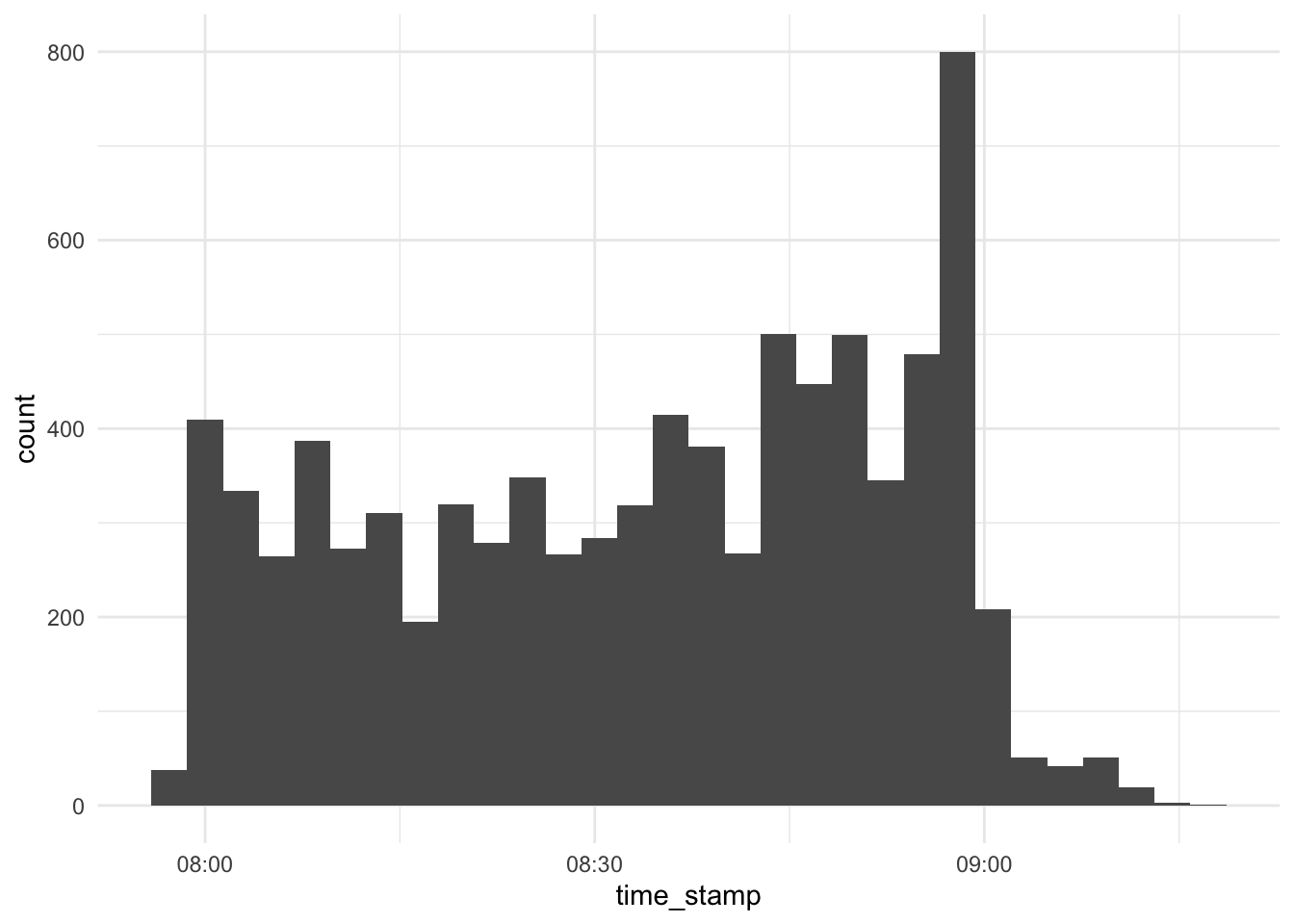
Hm…
d_exam1 %>%
  select(time_stamp) %>%
  ggplot(aes(x = time_stamp)) +
  scale_x_datetime() +
  geom_density()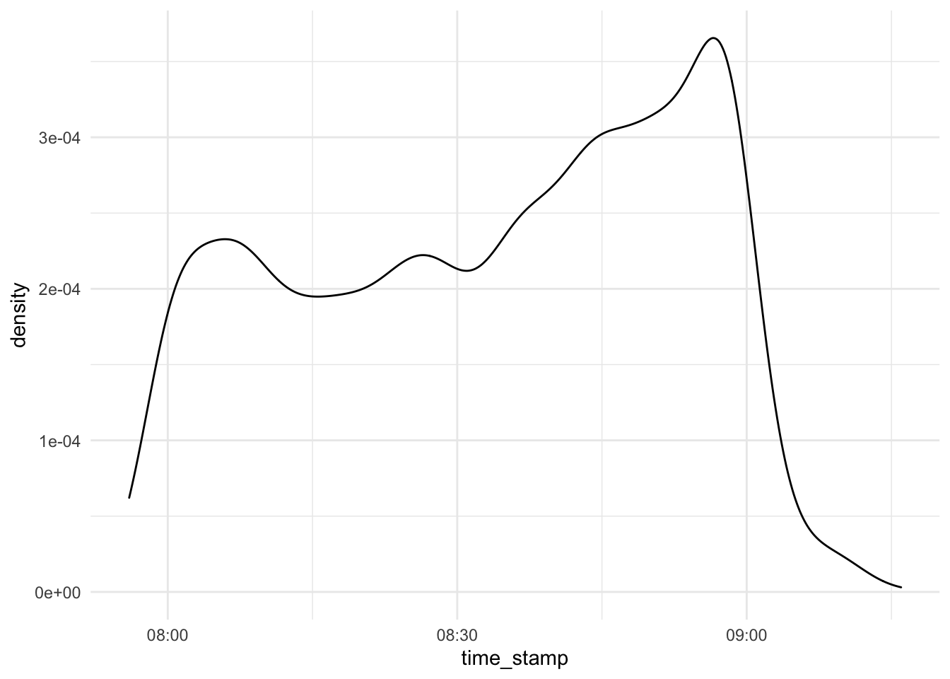
Looks unsuspicious.
Let’s depict each server interaction as a dot:
d_exam1 %>%
  cbind(y = runif(n = nrow(d_exam1))) %>%
  relocate(y, .before = 1) %>%
  relocate(time_stamp, .before = 2) %>%
  ggplot(aes(x = time_stamp, y = y)) +
  geom_point(alpha = .1) +
  scale_x_datetime() +
  scale_y_continuous(limits = c(0, 1))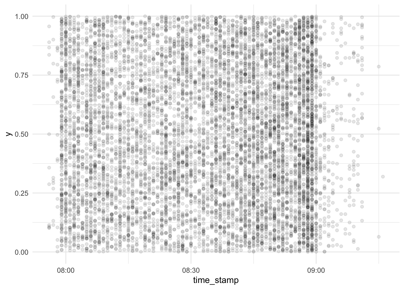
Let’s zoom in right before the end of the test:
d_exam1 %>%
  cbind(y = runif(n = nrow(d_exam1))) %>%
  relocate(y, .before = 1) %>%
  relocate(time_stamp, .before = 2) %>%
  ggplot(aes(x = time_stamp, y = y)) +
  geom_point(alpha = .1) +
  scale_x_datetime(limits = c(ymd_hm("2022-01-31 08:50"), ymd_hm("2022-01-31 09:00"))) +
  scale_y_continuous(limits = c(0, 1))
## Warning: Removed 6447 rows containing missing values (geom_point).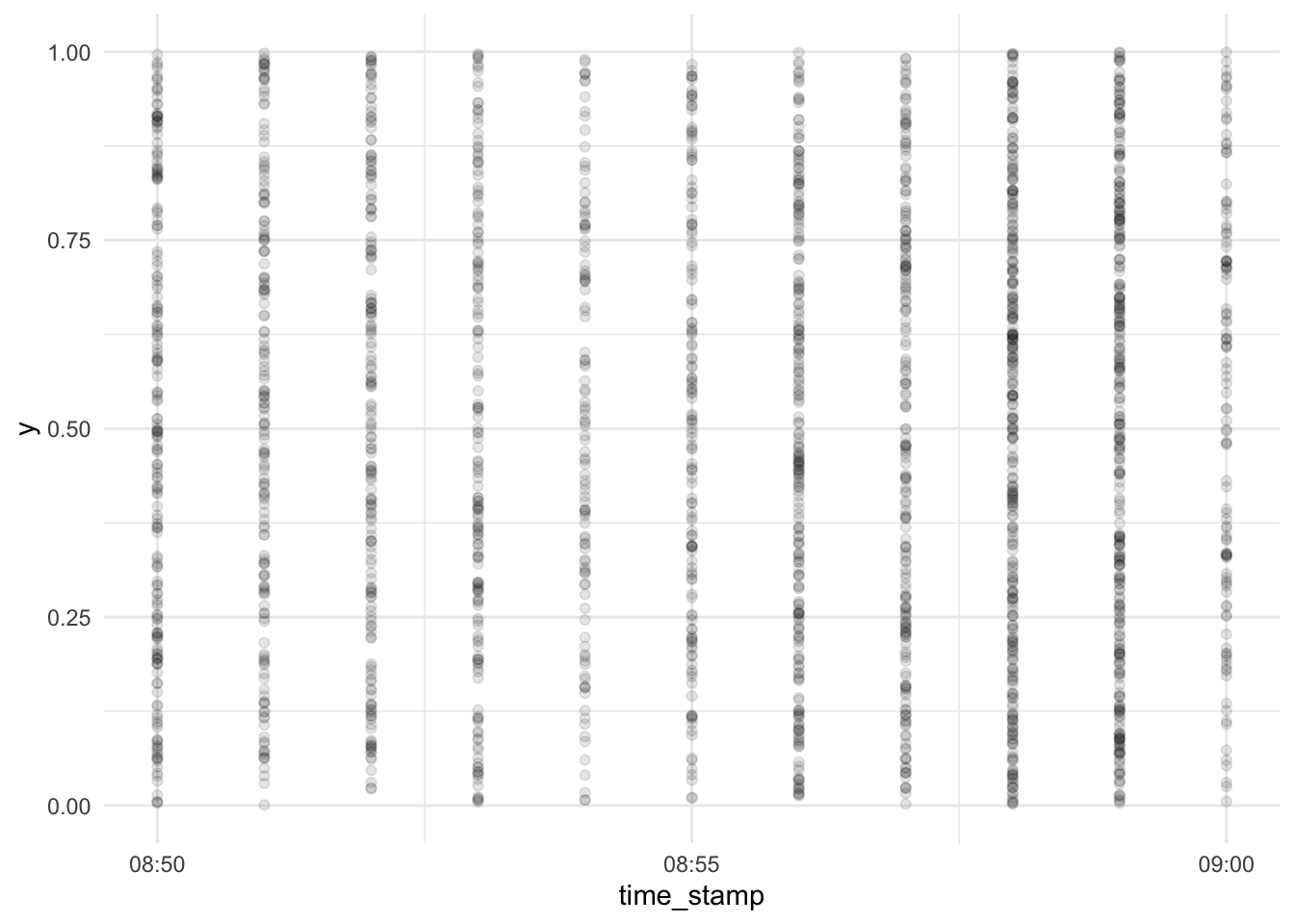
It appears the time wise resolution of our data does not allow for finer grains than 1 one minute windows.
Let’s try something more quantitatively looking:
d_exam1 %>%
  select(time_stamp) %>%
  filter(between(time_stamp, ymd_hm("2022-01-31 08:00"), ymd_hm("2022-01-31 08:59"))) %>%
  count(time_stamp) %>%
  ggplot() +
  geom_col(aes(x = time_stamp, y = n))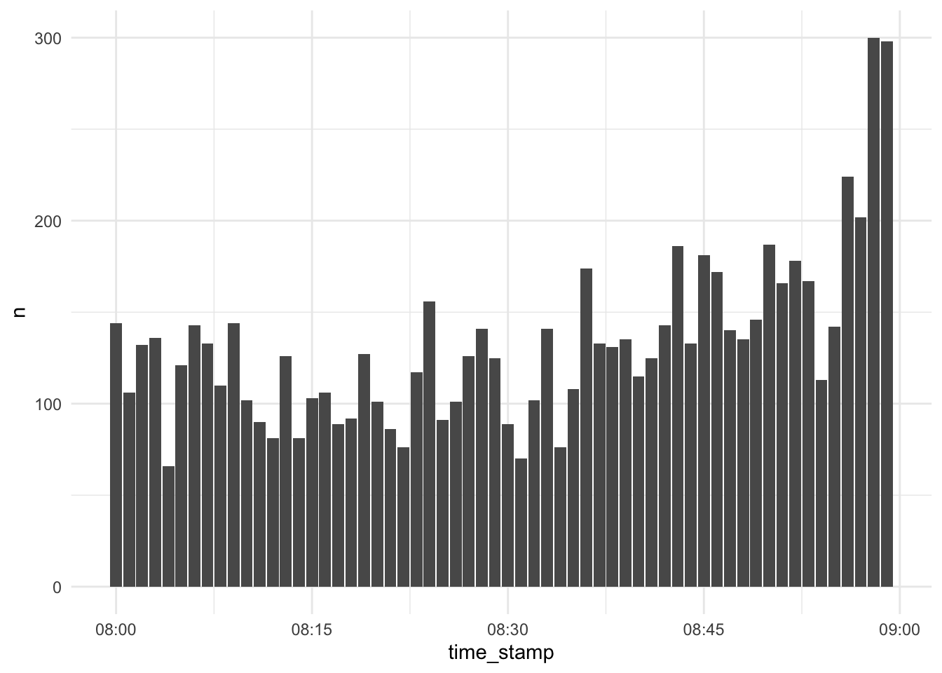
Looks unsuspicious.
Debrief
Not finding evidence of some failure is not evidence of no failure, in general at least.