Confounder

A confounder is on of the few (maybe three) “atoms” of causality, following the framework of Judea Parl and others.

A confounder can be depicted like this:

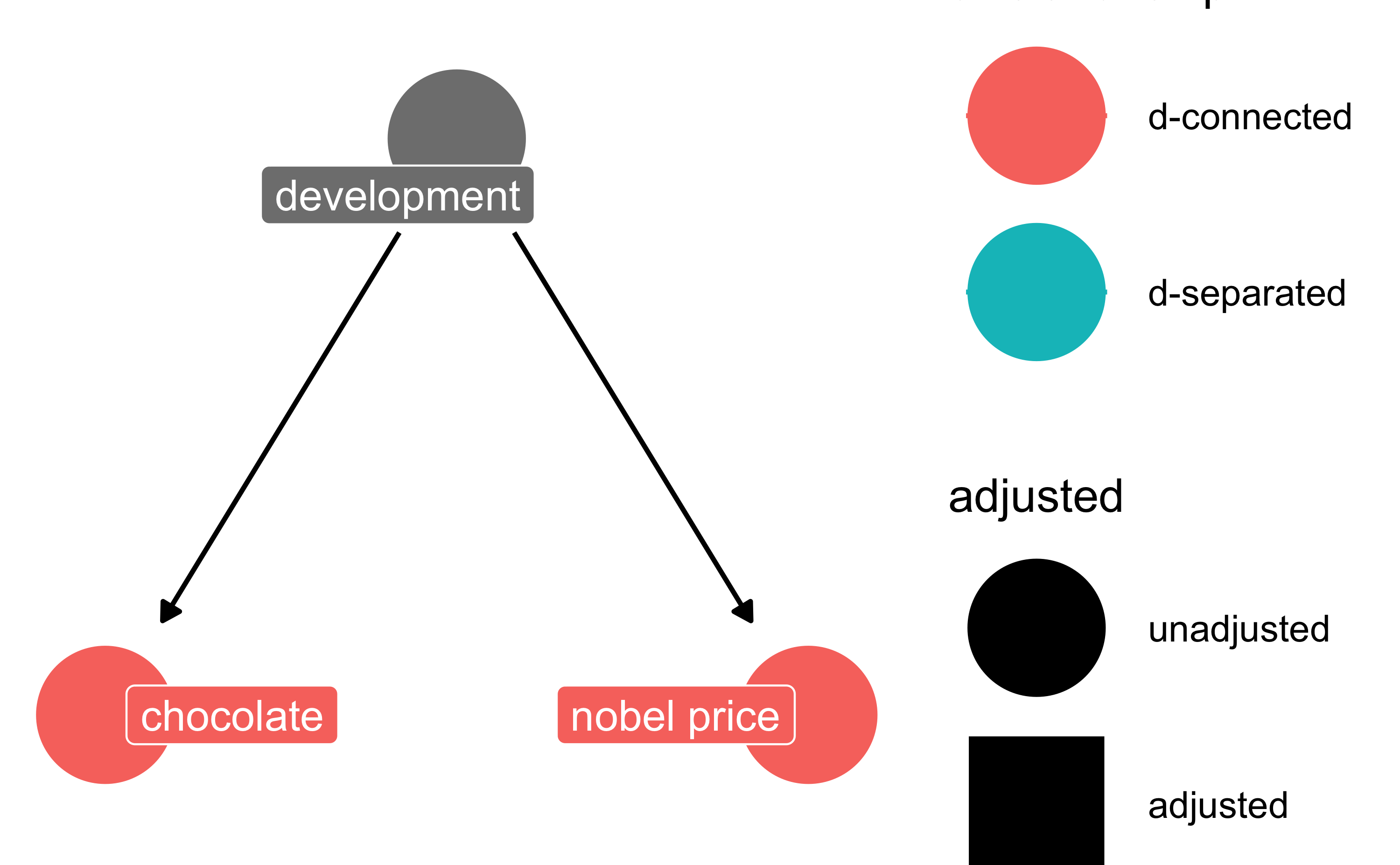
Following a study that reported a strong correlation between chocolate consumption and Nobel prices.

Simulating a confounder structure

Now let’s simulate a simple confounder structure.

Here’s some code that will help us:

Let’s have a look at the code:

## 
## n <- 100
## 
## set.seed(42)
## 
## d_sim <-
##   tibble(
##     x = rnorm(n, 0, 0.5),
##     y = rnorm(n, 0, 0.5),
##     group = "A"
##   ) %>%
##   bind_rows(
##     tibble(
##       x = rnorm(n, 1, 0.5),
##       y = rnorm(n, 1, 0.5),
##       group = "B")
##   )
## 
## 
## p_konf1 <-
##   d_sim %>%
##   ggplot(aes(x = x, y = y)) +
##   geom_point() +
##   geom_smooth(method = "lm") +
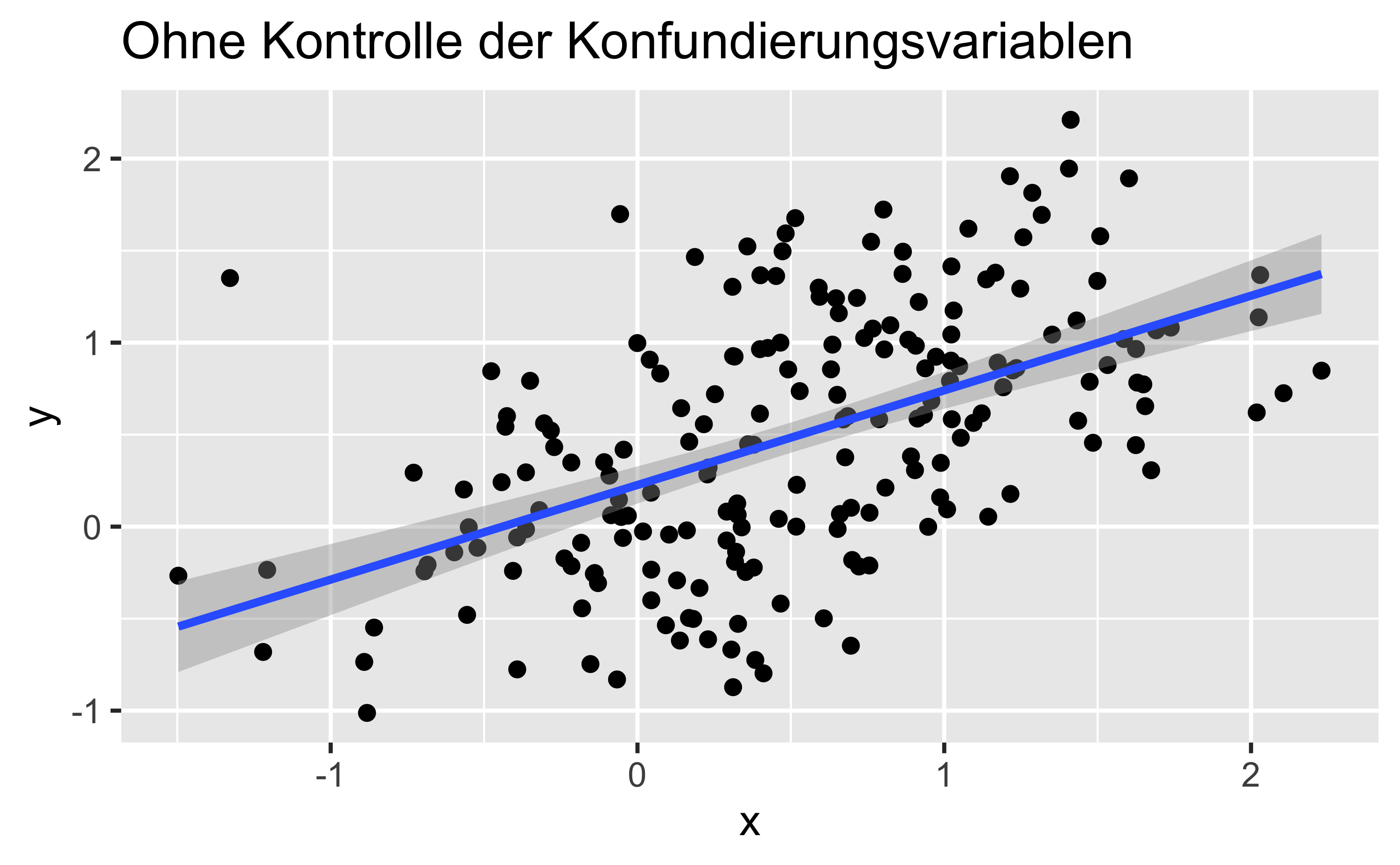
##   labs(title = "Ohne Kontrolle der Konfundierungsvariablen")
## 
## p_konf2 <-
##   d_sim %>%
##   ggplot(aes(x = x, y = y, color = group)) +
##   geom_point() +
##   geom_smooth(method = "lm") +
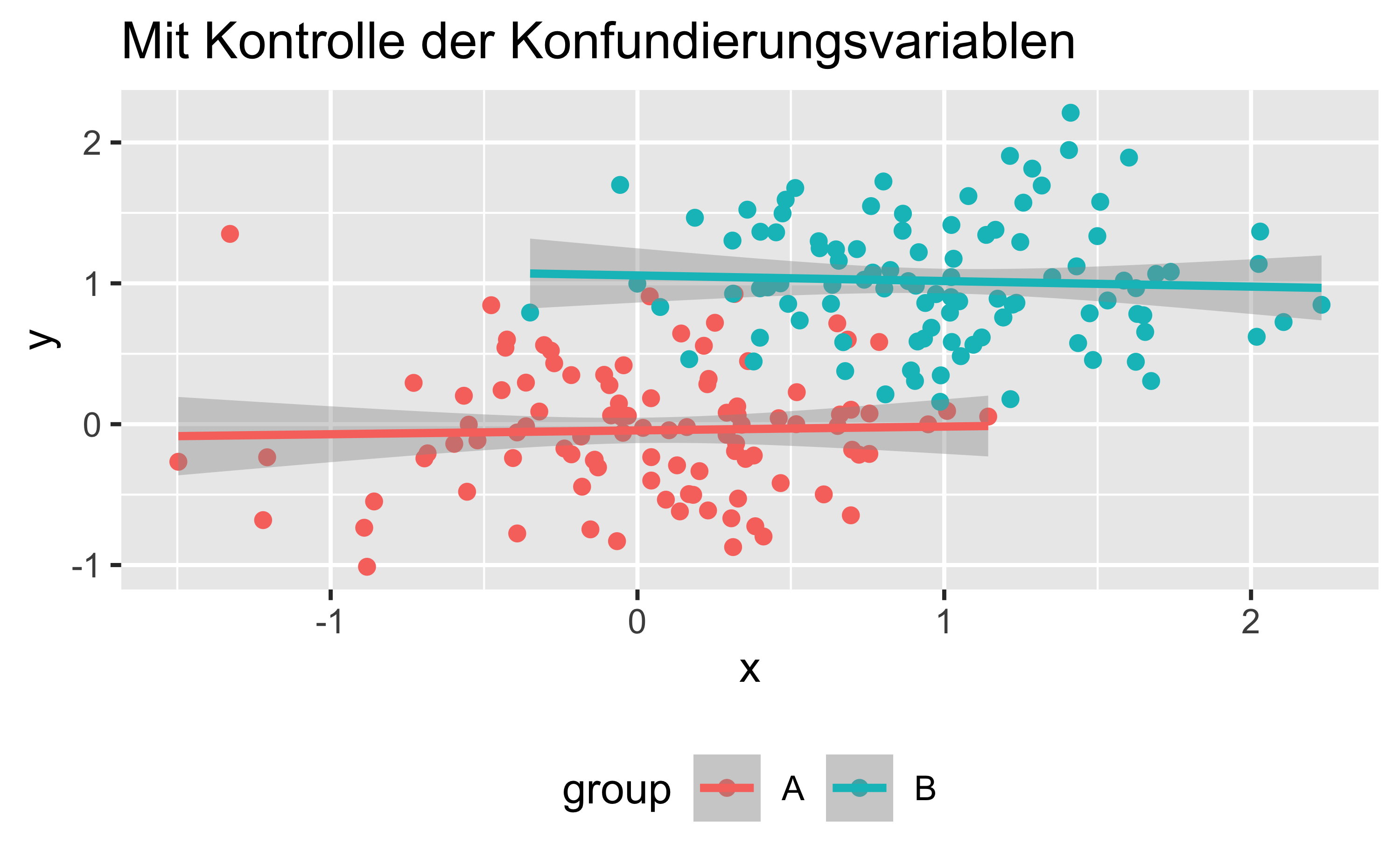
##   labs(title = "Mit Kontrolle der Konfundierungsvariablen") +
##   theme(legend.position = "bottom")

Here are the plots: