1 Exemplary Research question

What is the sample size needed to estimate the proportion of the event “high quality study” with an error margin of ±5%, and a confidence level of 99%? Let’s assume the probability of the event is 50%, and we draw the studies independently?

2 Task definition

Let’s simulate the width of a \(1-\alpha\) compatibility interval with a given margin of error \(E\) for varying samples sizes \(n_i\), where \(i = 1,...,N\), and \(N\) is the maximum sample size we can afford. We’ll assume indendently distributed and independent trials (iid).

Let’s further assume we are looking at a binary event \(X\) with a success \(x\) probability of \(Pr(X=x)=p\).

Let \(Y_k = \sum_1^i X_j\); think of \(Y_k\) as one sample of a given sample size, \(n_i\). Note that \(Y_k \overset{iid}{\sim} \mathcal{B}(n,p)\) (Binomially distributed).

Let’s draw \(K\) samples for each \(Y_k\), and dub the resulting statistic \(Z_i\). We’ll compute \(Z_i\) for each sample size \(n_i\), with \(i = 1,...,N\).

Finally, we’ll compute the arithmetic average of each \(Y_k\) and of \(Z_i\), for scale independency.

3 Technical setup

We’ll run this simulation in R, making use of the following packages:

library(tidyverse)
library(scales)
library(glue)
library(moments)

4 Define constants

N <- 1e04  # max. sample size
E <- .05  # error margin
p <- 1/2  # probability of event (success)
alpha = .01  # compatibility level
K <- 1e03  # repetitions per sample size

q <- abs(qnorm(p = alpha/2))
q  # quantile in the normal distribution for alpha

## [1] 2.575829

Note that \(p=1/2\) is the maximum conservative assumption yielding the largest sample size.

5 Prepare data frame for the simulation

df <- tibble(
  i = 1:N,
  estimate = NA,
  se = NA,
  lwr = NA,
  upr = NA,
  width = NA,
  small_enough = NA
)

6 Simulation

Let’s draw \(N\) samples with increasing sample size from 1 to \(N=10^{4}\), each time with \(K=1000\) repetitions, assuming independent draws and a Binomial distribution with \(p=0.5\).

for (i in 1:N) {
  # draw K "coin flip" samples of size i, 
  # with succcess propability p: 
  tmp <- rbinom(n = K, size = i, prob = p)
  # compute succcess rate for each sample:
  prop_success <- tmp/i
  # compute success rate over all K samples:
  df$estimate[i] <- mean(prop_success)
  # compute standard error:
  df$se[i] <- sd(prop_success)
  # compute interval borders and width:
  df$lwr[i] <- df$estimate[i] - q * df$se[i]
  df$upr[i] <- df$estimate[i] + q * df$se[i]
  df$width[i] <- df$upr[i] - df$lwr[i] 
  # check if intervals is as small as desired:
  if (df$width[i] < 2*E)
   {df$small_enough[i] <- TRUE} else {
     df$small_enough[i] <- FALSE}
}

7 Check some distributions

Note that the binomial distributions converges against the normal distribution. For instance, let’s pick \(n_i=100\) and \(K=10^4\).

smple <- tibble(
 estimate = rbinom(n = 1e04, 
                   size = 100, 
                   prob = p))

smple %>% 
  ggplot(aes(x = estimate)) +
  geom_density()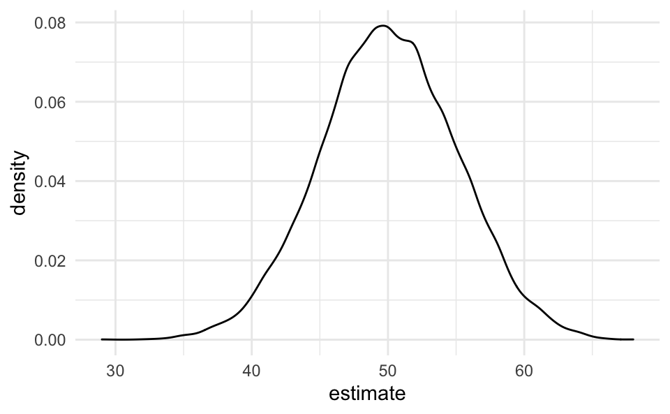

Let’s briefly check for normality, using a quantile-quantile plot:

ggplot(smple, aes(sample = estimate)) + 
  stat_qq() +
  stat_qq_line(col = "red")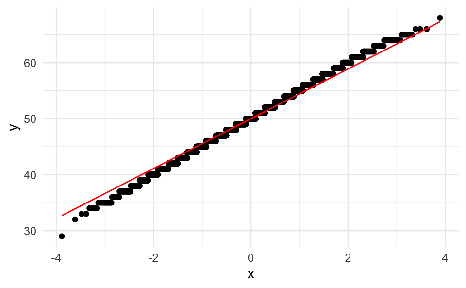

This check reassured us that this distribution is normal.

Add some stats for checking normality:

skewness(smple$estimate)

## [1] -0.01740677

kurtosis(smple$estimate)

## [1] 2.952453

Which nicely fits a normal distribution.

Also note that a linear transformation of a normal curve is still normal:

tibble(
 estimate = rbinom(n = 1e04, 
                   size = 100, 
                   prob = p),
 prop = estimate / 100) %>% 
  ggplot(aes(x = prop)) +
  geom_density()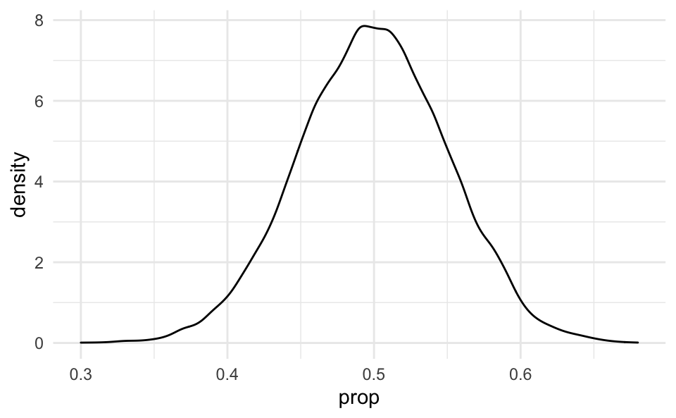

8 Minimum sample size

What’s the minimum sample size \(n_{min}\) needed such that \(w \le 2E\), where \(w\) denotes the width of the compatibility interval?

n_min <- 
  df$width %>% 
  detect_index(~ .x <= 2*E)

n_min

## [1] 357

What’s the maximum sample size \(n_{max}\) needed such that \(w > 2E\)?

n_max <- 
  df$width %>% 
  detect_index(~ .x > 2*E, .dir = "backward")

n_max

## [1] 419

9 Plot results

df %>% 
  filter(i > 30) %>% 
  ggplot(aes(x = i, y = width)) +
  geom_line() + 
  scale_x_continuous(trans = log10_trans()) + 
  geom_hline(yintercept = 2*E, linetype ="dashed", color = "grey60") +
  annotate("label", x = 100, y = .1, label = "2E") +
  geom_vline(xintercept = n_max, linetype = "dashed", 
             color = "blue") +
  geom_vline(xintercept = n_min, linetype = "dashed",
             color = "red") +
  annotate("label", x = n_max, y = .3, 
           label = glue("nmax={n_max}"), 
           color = "blue") +
  annotate("label", x = n_max, y = .2, 
           label = glue("nmin={n_min}"),
           color = "red") +
  labs(x = "sample size (log)",
       y = "margin of error",
       subtitle = "for estimating the width of compatibility intervals",
       title = "Simulating minimum sample sizes",
       caption = glue("Alpha: {alpha}, desired E = {E}, p = 1/2. See text for details.\n Each x-value depicts the average of {K} samples")) +
  theme_minimal()

10 Summary

The simulation implies that we need a sample size \(n\) of approx. around 357 to 419 to get a compatibility interval of width \(2E\) for an alpha level of \(1-\alpha=0.99\).

11 Discussion

This post proposes a rough approach of attaining practical sample sizes when an analytical approach is not wanted or feasible. Several limitations should be put forward: One might want with finite populations; one might want to compare the simulation results with typical formulas; one might prefer different stopping rules.

12 Suggested reading

Check out the following sources for related issues and more in-depth treatment: Landau and Stahl (2013), Schönbrodt and Perugini (2013), Maxwell, Kelley, and Rausch (2008), Arnold et al. (2011), Kruschke (2015).