1 Einführung

Dieser Post stellt den Code zum Kapitel 3 aus ARM vor, und zwar im Tidyverse-Stil.

2 Pakete laden

library(tidyverse)
library(arm)
library(foreign)
library(modelr)
library(ggfortify)

3 Daten laden

Die Daten können hier heruntergeladen werden als Zip-Datei. Danach muss man lokal entzippen und den Pfad am eigenen Rechner nennen. Tipp: Die Datendatei in den gleichen Ordner legen wie die Rmd-Datei; das erspart Rätseln über den korrekten Pfad.

kidsiq_path <- "/Users/sebastiansaueruser/datasets/ARM_Data/child.iq/kidiq.dta"

Die Daten sind im Format der Statistik-Software Stata gespeichert (.dta). Mit dem Paket foreign kann man solche Daten importieren.

kidsiq <- read.dta(kidsiq_path)

kidsiq %>% 
  slice_head(n=5)

##   kid_score mom_hs    mom_iq mom_work mom_age
## 1        65      1 121.11753        4      27
## 2        98      1  89.36188        4      25
## 3        85      1 115.44316        4      27
## 4        83      1  99.44964        3      25
## 5       115      1  92.74571        4      27

4 Ein Prädiktor

4.1 lm1: Binärer Prädiktor

lm1 <- lm (kid_score ~ mom_hs, data = kidsiq)
display(lm1)

## lm(formula = kid_score ~ mom_hs, data = kidsiq)
##             coef.est coef.se
## (Intercept) 77.55     2.06  
## mom_hs      11.77     2.32  
## ---
## n = 434, k = 2
## residual sd = 19.85, R-Squared = 0.06

4.1.1 Diagramm

kidsiq %>% 
  ggplot(aes(x = mom_hs, y = kid_score)) +
  geom_jitter(width = 0.2) +
  geom_smooth(method = "lm", se = FALSE) +
  scale_x_continuous(breaks = c(0, 1))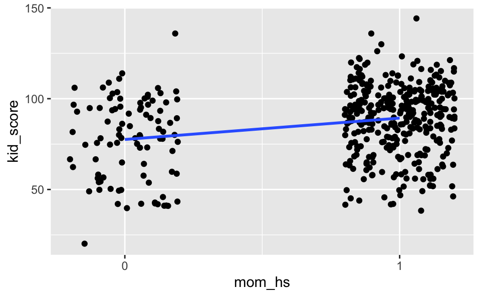

4.1.2 Unterschied im Mittelwert

kidsiq_summary <- 
  kidsiq %>% 
  group_by(mom_hs) %>% 
  summarise(kid_score = mean(kid_score, na.rm = TRUE))

kidsiq_summary

## # A tibble: 2 x 2
##   mom_hs kid_score
##    <dbl>     <dbl>
## 1      0      77.5
## 2      1      89.3

Differenz der Mittelwerte:

kidsiq_summary %>% 
  summarise(kid_score[1] - kid_score[2])

## # A tibble: 1 x 1
##   `kid_score[1] - kid_score[2]`
##                           <dbl>
## 1                         -11.8

Das entspricht der Steigung von lm1:

coef(lm1)

## (Intercept)      mom_hs 
##    77.54839    11.77126

4.2 lm2: Ein kontinuierlicher Prädiktor

lm2 <- lm(kid_score ~ mom_iq, data = kidsiq)
display(lm2)

## lm(formula = kid_score ~ mom_iq, data = kidsiq)
##             coef.est coef.se
## (Intercept) 25.80     5.92  
## mom_iq       0.61     0.06  
## ---
## n = 434, k = 2
## residual sd = 18.27, R-Squared = 0.20

ggplot(kidsiq) +
  aes(x = mom_iq, y = kid_score) +
  geom_point() +
  geom_abline(intercept = 25.8, slope = 0.61, color = "blue")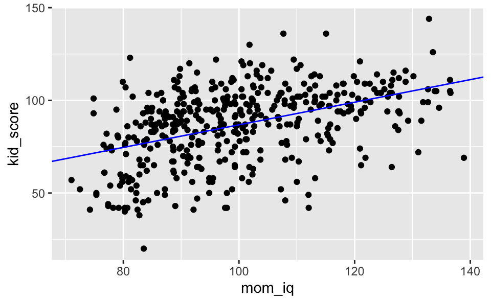

Oder so:

ggplot(kidsiq) +
  aes(x = mom_iq, y = kid_score) +
  geom_point() +
  geom_smooth(method = "lm", se = FALSE)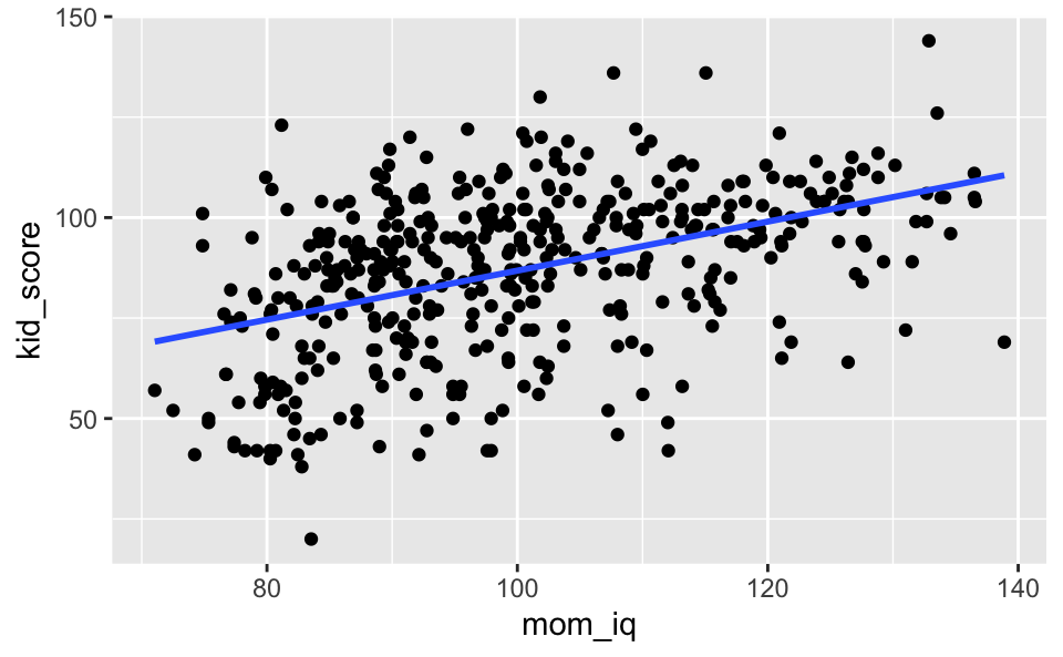

5 Mehrere Prädiktoren

5.1 lm3: Ohne Interaktionseffekt

lm3 <- lm(kid_score ~ mom_hs + mom_iq, data = kidsiq)
display(lm3)

## lm(formula = kid_score ~ mom_hs + mom_iq, data = kidsiq)
##             coef.est coef.se
## (Intercept) 25.73     5.88  
## mom_hs       5.95     2.21  
## mom_iq       0.56     0.06  
## ---
## n = 434, k = 3
## residual sd = 18.14, R-Squared = 0.21

kidsiq %>% 
  mutate(mom_hs = factor(mom_hs)) %>% 
  ggplot() +
  aes(x = mom_iq, y = kid_score, group = mom_hs) +
  geom_point() +
  geom_abline(slope = 0.56, intercept = 25.73, color = "grey20") +
  geom_abline(slope = 0.56, intercept = 25.73+5.95, color = "red")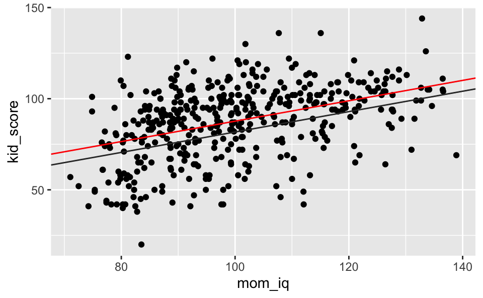

5.2 lm4: Mit Interaktionseffekt

lm4 <- lm(kid_score ~ mom_hs + mom_iq + mom_hs:mom_iq, data = kidsiq)
display(lm4)

## lm(formula = kid_score ~ mom_hs + mom_iq + mom_hs:mom_iq, data = kidsiq)
##               coef.est coef.se
## (Intercept)   -11.48    13.76 
## mom_hs         51.27    15.34 
## mom_iq          0.97     0.15 
## mom_hs:mom_iq  -0.48     0.16 
## ---
## n = 434, k = 4
## residual sd = 17.97, R-Squared = 0.23

kidsiq %>% 
  mutate(mom_hs = factor(mom_hs)) %>% 
  ggplot() +
  aes(x = mom_iq, y = kid_score, group = mom_hs) +
  geom_point() +
  geom_abline(slope = 0.97, intercept = -11.48, color = "grey20") +
  geom_abline(slope = 0.97-0.48, intercept = -11.48+51.27, color = "red")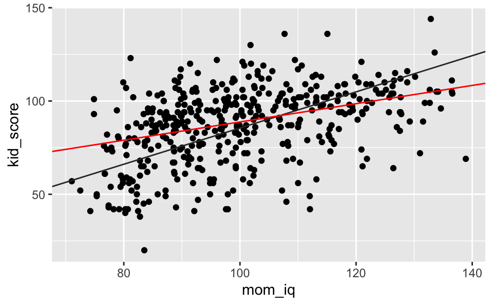

Oder so:

kidsiq %>% 
  mutate(mom_hs = factor(mom_hs)) %>% 
  ggplot() +
  aes(x = mom_iq, y = kid_score, group = mom_hs) +
  geom_point() +
  geom_smooth(aes(color = mom_hs),
              method = "lm", se = FALSE)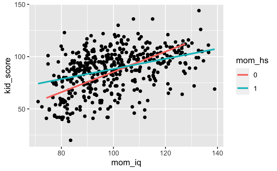

Mit Verlängerung der X-Achse zum Achsenabschnitt:

kidsiq %>% 
  mutate(mom_hs = factor(mom_hs)) %>% 
  ggplot() +
  aes(x = mom_iq, y = kid_score, group = mom_hs) +
  geom_point() +
  geom_abline(slope = 0.97, intercept = -11.48, color = "grey20") +
  geom_abline(slope = 0.97-0.48, intercept = -11.48+51.27, color = "red") +
  lims(x = c(0, 150), y = c(-20, 150))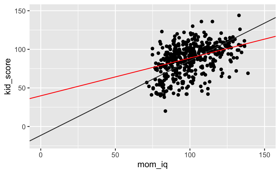

6 Eingeschränkter Wertebereich

kidsiq %>% 
  summarise(max_mom_iq = max(mom_iq),
            min_mom_iq = min(mom_iq))

##   max_mom_iq min_mom_iq
## 1   138.8931   71.03741

6.1 lm5: Regressionsmodell

lm5 <-
  kidsiq %>% 
  filter(mom_iq >= 85 & mom_iq <= 115) %>% 
  lm(kid_score ~ mom_iq, data = .)

display(lm5)

## lm(formula = kid_score ~ mom_iq, data = .)
##             coef.est coef.se
## (Intercept) 43.37    13.22  
## mom_iq       0.46     0.13  
## ---
## n = 277, k = 2
## residual sd = 18.14, R-Squared = 0.04

Vergleich mit uneingeschränktem Wertebereich:

display(lm2)

## lm(formula = kid_score ~ mom_iq, data = kidsiq)
##             coef.est coef.se
## (Intercept) 25.80     5.92  
## mom_iq       0.61     0.06  
## ---
## n = 434, k = 2
## residual sd = 18.27, R-Squared = 0.20

kidsiq %>% 
  filter(mom_iq >= 85 & mom_iq <= 115) %>% 
  ggplot() +
  aes(x = mom_iq, y = kid_score) +
  geom_point() +
  geom_abline(intercept = 25.8, slope = 0.61, color = "blue") +
  lims(x = c(70, 140))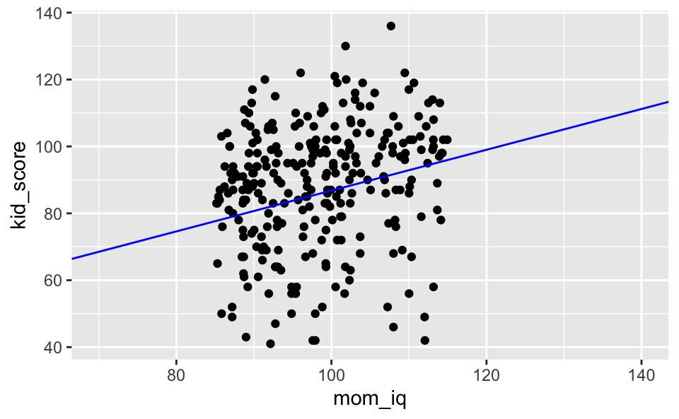

7 Visualisierung von Ungewissheit im Model

Der Standardfehler se ist ein Maß für unsere Ungewissheit in der Regressionsgeraden:

ggplot(kidsiq) +
  aes(x = mom_iq, y = kid_score) +
  geom_point() +
  geom_smooth(method = "lm", se = TRUE)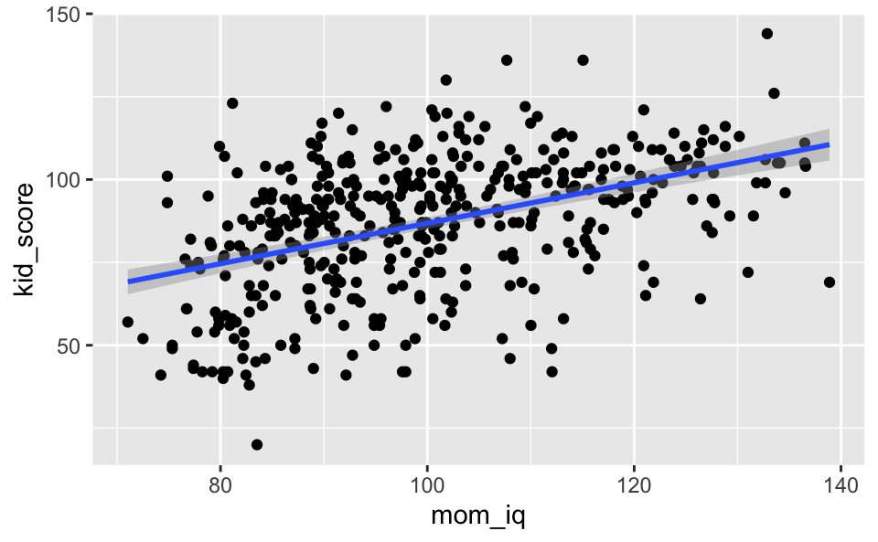

7.1 Variation eines Prädiktors und anderen konstant gehalten

7.1.1 Variation von `mom_iq`

Und mom_hs halten wir auf dem Mittelwert konstant:

kidsiq %>% 
  summarise(mean(mom_hs))

##   mean(mom_hs)
## 1    0.7857143

Ohne Visualisierung der Ungewissheit des Modells, nur mit einem Prädiktor auf dem Mittelwert fixiert:

kidsiq %>% 
  data_grid(mom_iq = seq_range(mom_iq, n = 20)) %>% 
  mutate(mom_hs = 0.79) %>% 
  add_predictions(lm3) %>% 
  ggplot(aes(x = mom_iq)) +
  geom_point(data = kidsiq, aes(y = kid_score)) +
  geom_line(aes(y = pred), color = "red")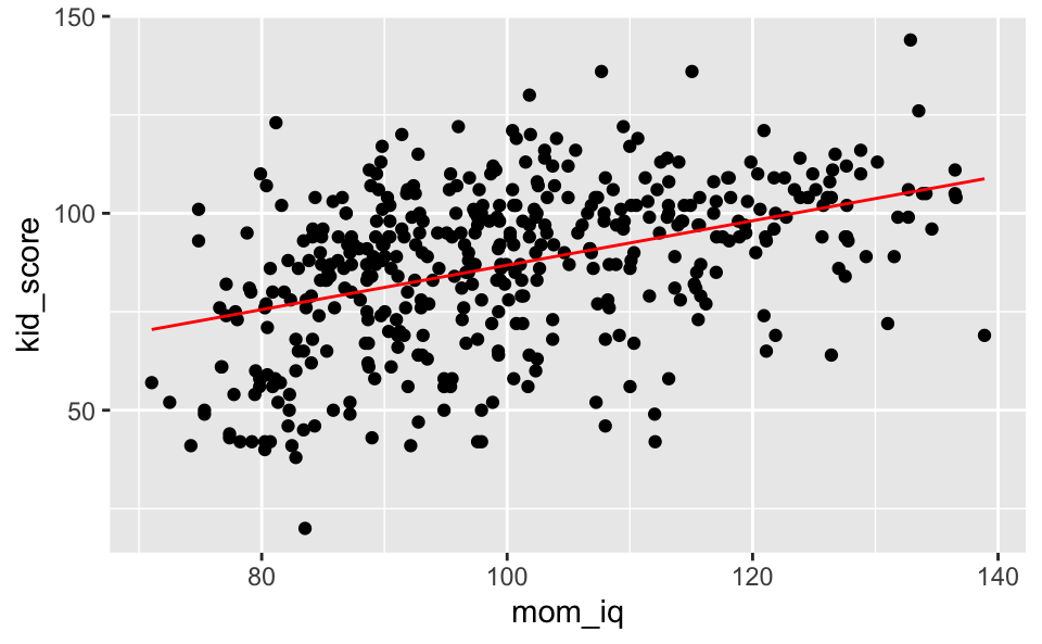

Oder so, jetzt auch mit Visualisierung des Standardfehlers, also mit Visualisierung der Ungewissheit des Modells:

kidsiq %>% 
  mutate(mom_hs = .79) %>% 
  ggplot(aes(x = mom_iq, y = kid_score)) +
  geom_point() +
  geom_smooth(method = "lm") +
  labs(title = "Zusammenhang (Kovariation) von mom_iq und kid_score\nwenn die übrigen Prädiktoren konstant gehalten sind (auf dem Mittelwert)")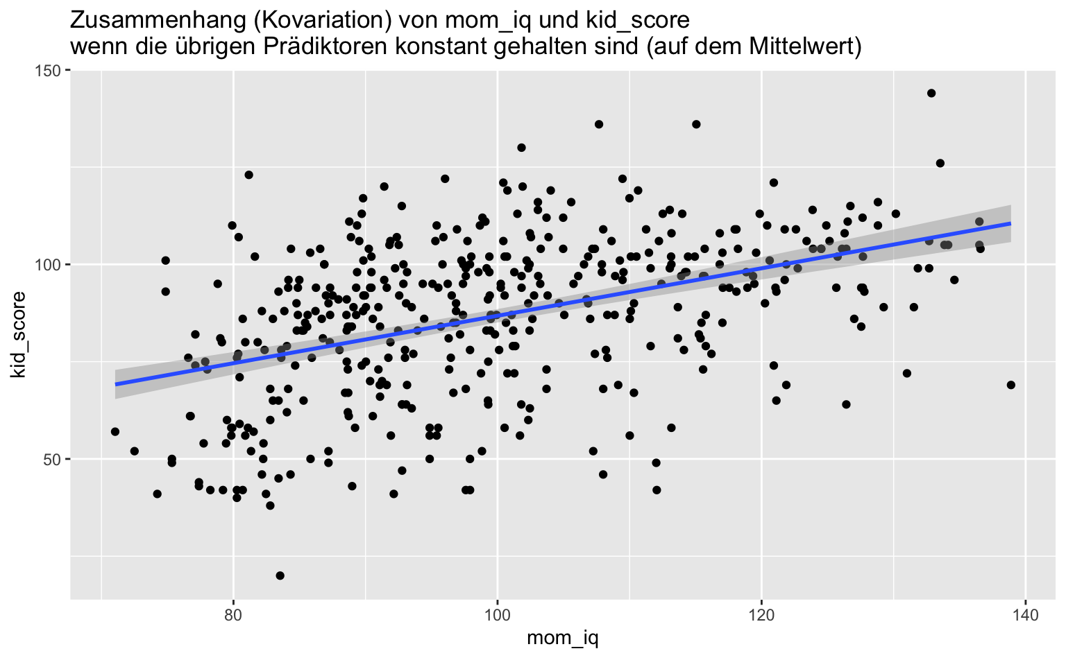

7.1.2 Kovariation mit `mom_iq`

kidsiq %>% 
  summarise(mean(mom_iq))

##   mean(mom_iq)
## 1          100

kidsiq %>% 
  mutate(mom_iq = 100) %>% 
  ggplot(aes(x = mom_hs, y = kid_score)) +
  geom_point() +
  geom_smooth(method = "lm") +
  labs(title = "Zusammenhang (Kovariation) von mom_hs und kid_score\nwenn die übrigen Prädiktoren konstant gehalten sind (auf dem Mittelwert)") +
  scale_x_continuous(breaks = c(0, 1)) +
  geom_label(data = kidsiq_summary,
    aes(label = round(kid_score, 2)))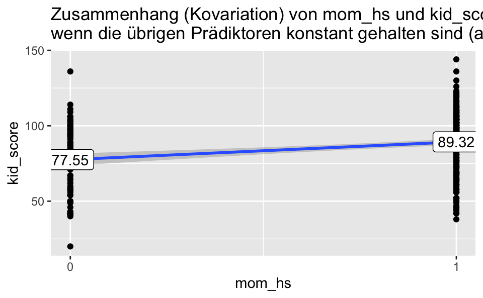

8 Annahmen der Regressionsanalyse

8.1 Additivität

\[\hat{y} = \beta_0 + \beta_1x_1 + \beta_2x_2 + \ldots\]

Bei Verletzung z.B.

8.1.1 Log-Transformation

\[y=abc \quad \leftrightarrow \quad \text{log} y = \text{log} a + \text{log} b + \text{log}\]

df <-
  tibble(
    x1 = 1:10,
    x2 = 1:10,
    x3 = 1:10,
    y = x1*x2*x3)

df %>% 
  mutate(y_log = x1 + x2 + x3)

## # A tibble: 10 x 5
##       x1    x2    x3     y y_log
##    <int> <int> <int> <int> <int>
##  1     1     1     1     1     3
##  2     2     2     2     8     6
##  3     3     3     3    27     9
##  4     4     4     4    64    12
##  5     5     5     5   125    15
##  6     6     6     6   216    18
##  7     7     7     7   343    21
##  8     8     8     8   512    24
##  9     9     9     9   729    27
## 10    10    10    10  1000    30

8.1.2 Interaktionen hinzufügen

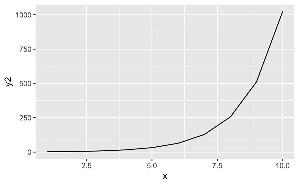
8.2 Linearität

Hier ist die Linearität verletzt:

df <-
  tibble(
    x = 1:10,
    y1 = x^2,
    y2 = 2^x)

df %>% 
  ggplot(aes(x = x, y = y1)) +
  geom_line()

df %>% 
  ggplot(aes(x = x, y = y2)) +
  geom_line()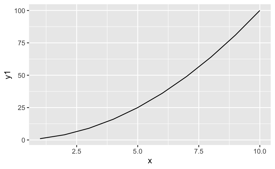

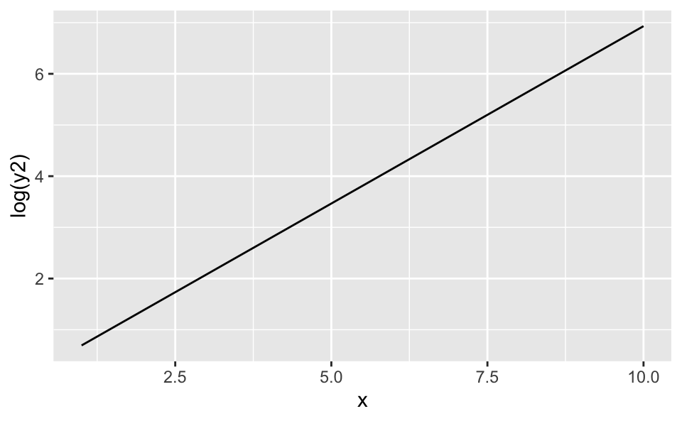
Durch eine passende Transformation kann die Linearität wieder hergestellt werden:

df %>% 
  ggplot(aes(x = x, y = sqrt(y1))) +
  geom_line()

df %>% 
  ggplot(aes(x = x, y = log(y2))) +
  geom_line()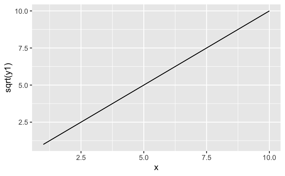

8.3 Visualisierung der Residen, um Verletzungen der Annahmen zu entdecken

8.4 Additivität

autoplot(lm3, which = 1)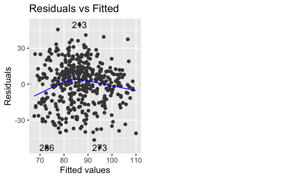

Wenn es keine Verletzungen gibt, sollten sich die Residen ohne Muster um die \(y=0\) herum verteilen. Hier sind die Residuen für mittlere Werte etwas erhöht und and den Randbereichen etwas zu gering. Insgesamt ist die Verletzung nicht gravierend.

8.5 Linearität

SD der Residuen

kidsiq %>% 
  add_residuals(lm2) %>% 
  summarise(sd(resid))

##   sd(resid)
## 1  18.24502

kidsiq %>% 
  add_residuals(lm2) %>% 
  ggplot(aes(x = mom_iq, y = resid)) +
  geom_ref_line(h = c(0)) +
  geom_hline(yintercept = c( -18, +18), 
             color = "grey60",
             linetype = "dashed") +
  geom_point() +
  labs(title = "Residuen vs. Prädiktor",
       caption = "Gestrichtelte Linien zeigen ±1SD")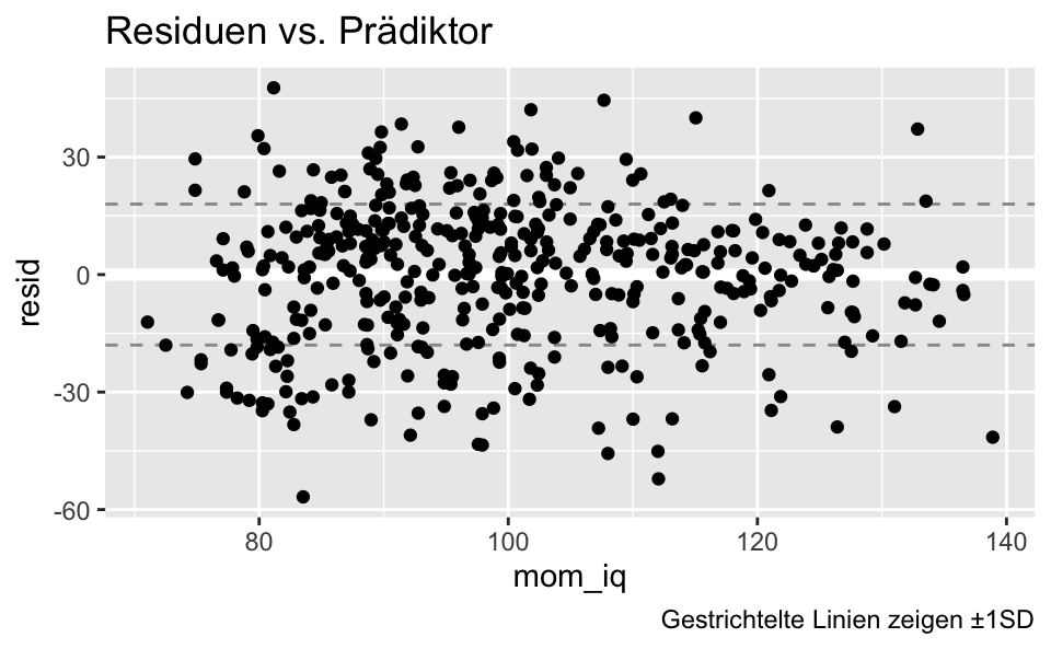

Hier zeigt sich nur Rauschen: Die Residuen sind ohne erkennbares Muster um \(y=0\) herum verteilt. Es ist keine Verletzung der Linearitätsannahme erkennbar.

9 Vorhersage

Nicht ausgeführt.

10 Referenz

S. auch den Post zu ARM, Kap. 4

ARM, Kap. 3 Syntax im Tidyverse-Stil