1 Load packages
library(tidyverse) # data wrangling2 Motivation
In some sense, science is about estimating the effect sizes in a population, such as . In the most basic form, perhaps, the question is nothing more than whether or not.
Given a population of limited size, we might be tempted to say, let’s measure all instances (such as individuals) of the population to come up wit the “real” . For concreteness, the population might consist of parts produced by some machine, or papers written by some scientists, which is the same for the question we are looking at now.
In this post, we will simulate the effect of sample sizes on population parameter estimates, in particular , but without of loss of generality, this applies to other type of population parameter in the same way. Of note, effect sizes can be converted from one to one other, such as , and the like.
3 True value of the parameter
Let’s decide on the true population parameter value. I argue that it is impossible, or at least unlikely, that the absolute value of this parameter is large. It it were large, we had no doubts about it. For instance, the effect size of water in the face of thirst is large. The effect of parachutes on falling speed is large. No need for estimating population parameter values.
For the sake of concreteness, I will speak of the “effectiveness of some medical intervention” in the following when I refer to the parameter value of .
On the other hand, if the value of the parameter is not large (in absolute terms), we arrive at the question whether the value is zero or not. I doubt that more precise values can be estimated in most practical cases. For example, to be confident that rather than (in SMD units) is beyond hope given the large amount of uncertainty we face even (or particularly) in modern science.
Hence, let’s assume that in the following. For the sake of simplicity, I will assume that the parameter under investigation is normally distributed. However, more ink could (and should) be spilled on this question.
mu <- 0.5As I think the uncertainty is large, we must allow for a relatively large standard deviation of the distribution of effects. Some reasons why I think the uncertainty in our population parameter value is lage include: publication bias, researcher degrees of freedom, variety in protocols and operationalization, plain errors in the course of a study, trickiness of nature, and more.
Hence, let’s take .
s <- 0.5In sum:
What is the probability to observere a sample value larger less than zero?
p0 <- pnorm(q = 0, mean = 0.5, sd = .5) %>% round(2)
p0
#> [1] 0.16
In other words, we think that the probability that equals to 0.16; let’s call it .
Given this model, we assume that the probability that the treatment is effective equals to , that is
p1 <- 1 - p0
p1
#> [1] 0.84
And so forth.
4 Drawing samples
Let’s draw multiple sample for different samples sizes and see how precisely we will measure the (true) population value. Than we can plot the precision of the population value estimation as a function of the sample size. In other words, we conduct some kind of power analysis.
5 Define some constants
Let’s define some auxiliary constants.
We’ll draw sample of a given size:
k <- 100Let’s check sample sizes according to the log 2 sequence:
x <- 1:15
n <- 2^x

n
#>  [1]     2     4     8    16    32    64   128   256   512  1024  2048  4096
#> [13]  8192 16384 32768
6 Simulating samples
6.1 SummayFunction to compute sample statistics
comp_sample_stats <- function(sample_size,
                              mu,
                              sigma) {
  # draws sample and computes summary stats

  sample_temp <- rnorm(n = sample_size,
                       mean = mu,
                       sd = sigma)
  sample_mean <- mean(sample_temp)
  sample_sd <- sd(sample_temp)
  sample_se <- sample_sd / sqrt(n)
  sample_ci_u <- sample_mean + 2 * sample_se
  sample_ci_l <- sample_mean - 2 * sample_se
  mu_in_ci <- (mu > sample_ci_l) & (mu < sample_ci_u)
  zero_in_ci <- (sample_ci_l < 0) & (sample_ci_u > 0)

  sample_stats <-
    tibble(
      avg = sample_mean,
      stddev = sample_sd,
      se = sample_se,
      ci_u = sample_ci_u,
      ci_l = sample_ci_l,
      mu_in_ci = mu_in_ci,
      zero_in_ci = zero_in_ci
    )

  return(sample_stats)
}
6.2 Run the function multiple () times
# sample_size <- 30  # delete me later!

comp_sample_stats_many_samples <-
  function(sample_size,
           mu,
           sigma,
           k  # number of repetitions
           ) {
  # draws sample and computes summary stats
  # for k multiples samples
  # of a fixed sample size

  many_samples_results <-
    1:k %>%
    map_dfr( ~ comp_sample_stats(sample_size = sample_size,
                             mu = mu,
                             sigma = s),
             .id = "id") %>%
    mutate(n = sample_size,
           id = as.numeric(id))

  return(many_samples_results)
  }
6.3 Run the summary function times for all sample sizes
simulated_samples <-
  n %>%
  map_dfr( ~ comp_sample_stats_many_samples(
    sample_size = .x,
    mu = mu,
    sigma = s,
    k = k)) %>%
    mutate(ci_width = ci_u - ci_l)
7 Plot the results
Remeber that all results presented here hinge of the assumption stated above. In particular, we have simulated samples.
7.1 Estimated population mean
p1 <- simulated_samples %>%
  ggplot() +
  aes(x = n, y = avg) +
  geom_jitter(alpha = .03)

p1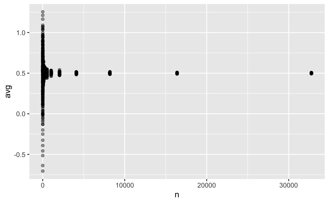
As can be seen, all sample sizes greater than small do precisely show the true parameter ().
Let’s zoom in.
p1 +
xlim(0, 1024)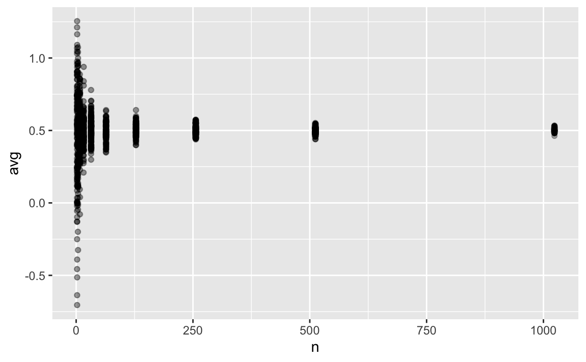 And even closer:
p1 +
  xlim(0, 256)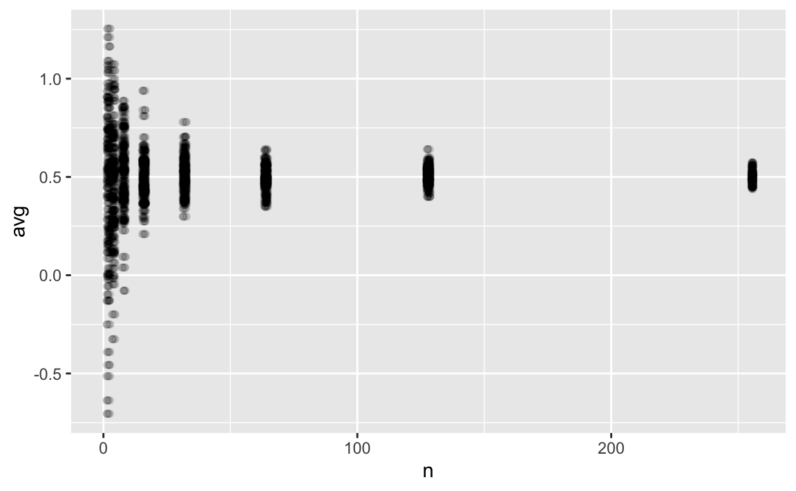
Larger sample sizes yield stable estimates, as seen above. But even the difference between and () appears negligible, from a practical point of view, given the large uncertainties associated with research study results in practice. Let’s remember that we should try to be more precise as it is possible (don’t estimate the age of the earth in seconds, rather in millions of years).
It appears that a sample size of 128 or even 64 is sufficiently precise to estimate the population effect size.
7.2 Width of the CI
p2 <- simulated_samples %>%
  ggplot() +
  aes(x = factor(n), y = ci_width) +
  geom_boxplot(aes(group = n))

p2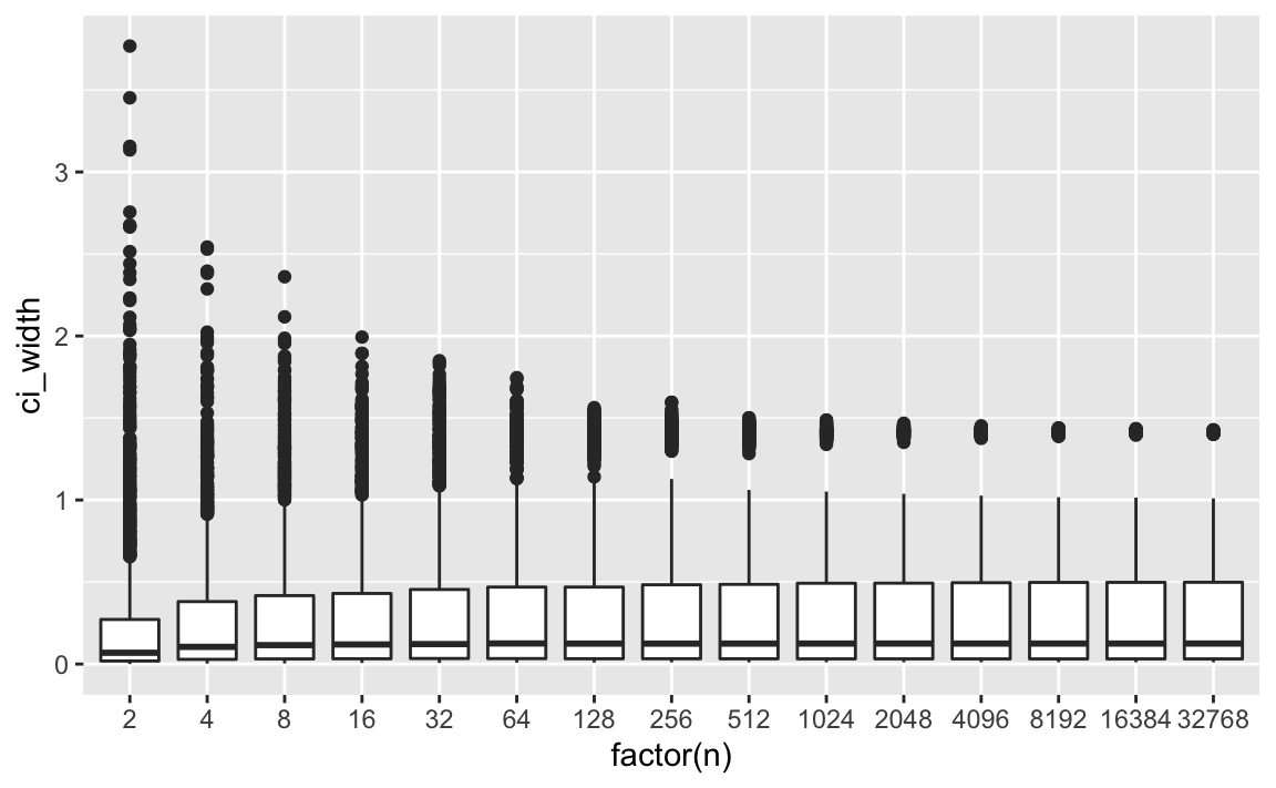
Again, zoom in:
p3 <- simulated_samples %>%
  filter(n <= 1024) %>%
  ggplot() +
  aes(x = factor(n), y = ci_width) +
  geom_boxplot(aes(group = n))

p3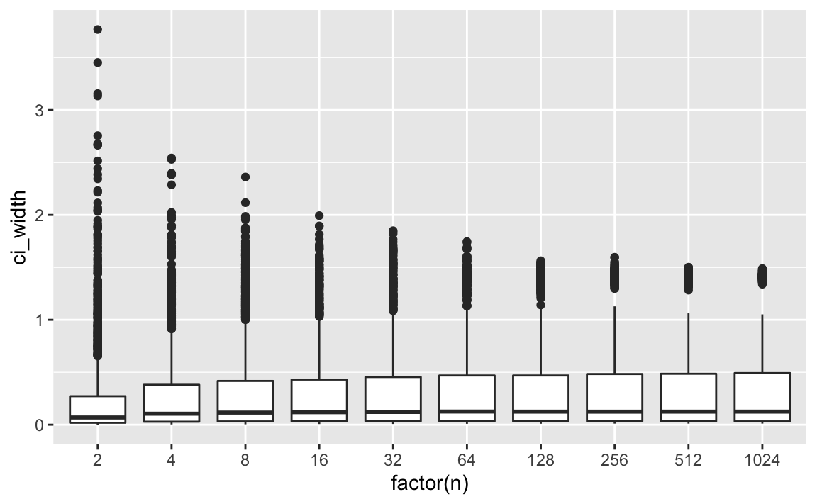
We can see that the width of the CI remains constant after an initial stabilizing phase. So, at say, we already have stable width estimates.
8 Summarise the results
8.1 Compute summaries per sample size
simulated_samples_summarized <- simulated_samples %>%
  group_by(n)  %>%
  summarise(across(
    .cols = everything(),
    .fn = list(avg = mean, sd = sd),
    .names = "{.col}_{.fn}"))

glimpse(simulated_samples_summarized)
#> Rows: 15
#> Columns: 19
#> $ n              <dbl> 2, 4, 8, 16, 32, 64, 128, 256, 512, 1024, 2048, 4096, 8…
#> $ id_avg         <dbl> 50.5, 50.5, 50.5, 50.5, 50.5, 50.5, 50.5, 50.5, 50.5, 5…
#> $ id_sd          <dbl> 28.8757, 28.8757, 28.8757, 28.8757, 28.8757, 28.8757, 2…
#> $ avg_avg        <dbl> 0.4641198, 0.4601394, 0.5191425, 0.4979736, 0.5113036, …
#> $ avg_sd         <dbl> 0.403764406, 0.271859795, 0.182014436, 0.115415684, 0.0…
#> $ stddev_avg     <dbl> 0.3901300, 0.4498725, 0.4770262, 0.4808355, 0.4969101, …
#> $ stddev_sd      <dbl> 0.291619823, 0.170001687, 0.126538119, 0.086169598, 0.0…
#> $ se_avg         <dbl> 0.06244360, 0.07200590, 0.07635208, 0.07696179, 0.07953…
#> $ se_sd          <dbl> 0.1091820, 0.1011893, 0.1020481, 0.0999563, 0.1023639, …
#> $ ci_u_avg       <dbl> 0.5890070, 0.6041512, 0.6718467, 0.6518971, 0.6703729, …
#> $ ci_u_sd        <dbl> 0.4627397, 0.3363836, 0.2745602, 0.2309151, 0.2234326, …
#> $ ci_l_avg       <dbl> 0.3392326, 0.3161276, 0.3664384, 0.3440500, 0.3522342, …
#> $ ci_l_sd        <dbl> 0.4552902, 0.3414320, 0.2723706, 0.2307593, 0.2240294, …
#> $ mu_in_ci_avg   <dbl> 0.2066667, 0.3120000, 0.3833333, 0.4840000, 0.5346667, …
#> $ mu_in_ci_sd    <dbl> 0.40504930, 0.46346435, 0.48636055, 0.49991060, 0.49896…
#> $ zero_in_ci_avg <dbl> 0.12000000, 0.13533333, 0.09466667, 0.09466667, 0.09466…
#> $ zero_in_ci_sd  <dbl> 0.3250699, 0.3421933, 0.2928516, 0.2928516, 0.2928516, …
#> $ ci_width_avg   <dbl> 0.2497744, 0.2880236, 0.3054083, 0.3078472, 0.3181386, …
#> $ ci_width_sd    <dbl> 0.4367281, 0.4047573, 0.4081926, 0.3998252, 0.4094558, …
8.2 Plot the (summarized) results
simulated_samples_summarized %>%
  ggplot() +
  aes(x = n, y = avg_avg,
      ymin = avg_avg - avg_sd,
      ymax = avg_avg + avg_sd
      ) +
  geom_ribbon(alpha = .5) +
  geom_point() +
  xlim(0, 128) +
  labs(x = "Sample size",
       y = "Average across 100 samples",
       caption = "The ribbon shows the interval [mean ± se]")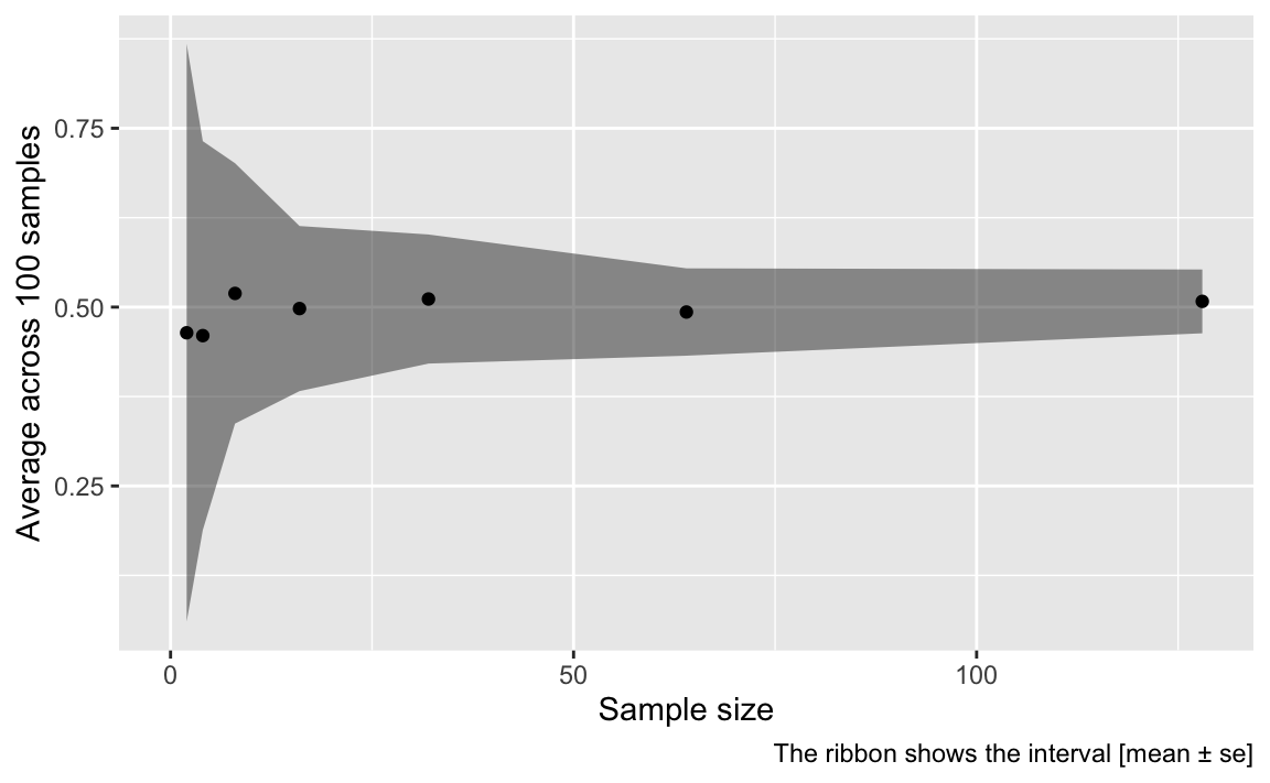
9 Conclusions
9.1 Small sample may suffice
Under well-defined situations such as the one presented here, small samples are sufficient.
However, it must be stressed that this comfortable conclusions hinges on the assumptions stated above.
9.2 Situations in which small samples will not suffice
The standard errors (for the mean value) increases as a function of variability (standard deviation, ie., sigma) in the population. The well-known formula for SE is valid only in the normal distribution scenario. If we assumed different distributions for the population parameter , we would arrive, in most situation, at much larger samples sizes. We might event encounter situations, such as for Cauchy distribution, where there are no mean values at all, and hence we are lost in complete ignorance about the precision of our estimates.
10 Reproducibility
#> ─ Session info ───────────────────────────────────────────────────────────────────────────────────────────────────────
#>  setting  value
#>  version  R version 4.0.2 (2020-06-22)
#>  os       macOS  10.16
#>  system   x86_64, darwin17.0
#>  ui       X11
#>  language (EN)
#>  collate  en_US.UTF-8
#>  ctype    en_US.UTF-8
#>  tz       Europe/Berlin
#>  date     2021-03-04
#>
#> ─ Packages ───────────────────────────────────────────────────────────────────────────────────────────────────────────
#>  package     * version     date       lib source
#>  assertthat    0.2.1       2019-03-21 [1] CRAN (R 4.0.0)
#>  backports     1.2.1       2020-12-09 [1] CRAN (R 4.0.2)
#>  blogdown      1.1         2021-01-19 [1] CRAN (R 4.0.2)
#>  bookdown      0.21.6      2021-02-02 [1] Github (rstudio/bookdown@6c7346a)
#>  broom         0.7.5       2021-02-19 [1] CRAN (R 4.0.2)
#>  bslib         0.2.4.9000  2021-02-02 [1] Github (rstudio/bslib@b3cd7a9)
#>  cachem        1.0.4       2021-02-13 [1] CRAN (R 4.0.2)
#>  callr         3.5.1       2020-10-13 [1] CRAN (R 4.0.2)
#>  cellranger    1.1.0       2016-07-27 [1] CRAN (R 4.0.0)
#>  cli           2.3.1       2021-02-23 [1] CRAN (R 4.0.2)
#>  codetools     0.2-16      2018-12-24 [2] CRAN (R 4.0.2)
#>  colorspace    2.0-0       2020-11-11 [1] CRAN (R 4.0.2)
#>  crayon        1.4.1       2021-02-08 [1] CRAN (R 4.0.2)
#>  DBI           1.1.1       2021-01-15 [1] CRAN (R 4.0.2)
#>  dbplyr        2.1.0       2021-02-03 [1] CRAN (R 4.0.2)
#>  debugme       1.1.0       2017-10-22 [1] CRAN (R 4.0.0)
#>  desc          1.2.0       2018-05-01 [1] CRAN (R 4.0.0)
#>  devtools      2.3.2       2020-09-18 [1] CRAN (R 4.0.2)
#>  digest        0.6.27      2020-10-24 [1] CRAN (R 4.0.2)
#>  dplyr       * 1.0.4       2021-02-02 [1] CRAN (R 4.0.2)
#>  ellipsis      0.3.1       2020-05-15 [1] CRAN (R 4.0.0)
#>  evaluate      0.14        2019-05-28 [1] CRAN (R 4.0.0)
#>  fansi         0.4.2       2021-01-15 [1] CRAN (R 4.0.2)
#>  farver        2.0.3       2020-01-16 [1] CRAN (R 4.0.0)
#>  fastmap       1.1.0       2021-01-25 [1] CRAN (R 4.0.2)
#>  forcats     * 0.5.1       2021-01-27 [1] CRAN (R 4.0.2)
#>  fs            1.5.0       2020-07-31 [1] CRAN (R 4.0.2)
#>  generics      0.1.0       2020-10-31 [1] CRAN (R 4.0.2)
#>  ggplot2     * 3.3.3       2020-12-30 [1] CRAN (R 4.0.2)
#>  glue          1.4.2       2020-08-27 [1] CRAN (R 4.0.2)
#>  gtable        0.3.0       2019-03-25 [1] CRAN (R 4.0.0)
#>  haven         2.3.1       2020-06-01 [1] CRAN (R 4.0.0)
#>  highr         0.8         2019-03-20 [1] CRAN (R 4.0.0)
#>  hms           1.0.0       2021-01-13 [1] CRAN (R 4.0.2)
#>  htmltools     0.5.1.1     2021-01-22 [1] CRAN (R 4.0.2)
#>  httr          1.4.2       2020-07-20 [1] CRAN (R 4.0.2)
#>  jquerylib     0.1.3       2020-12-17 [1] CRAN (R 4.0.2)
#>  jsonlite      1.7.2       2020-12-09 [1] CRAN (R 4.0.2)
#>  knitr         1.31        2021-01-27 [1] CRAN (R 4.0.2)
#>  labeling      0.4.2       2020-10-20 [1] CRAN (R 4.0.2)
#>  lifecycle     1.0.0       2021-02-15 [1] CRAN (R 4.0.2)
#>  lubridate     1.7.9.2     2020-11-13 [1] CRAN (R 4.0.2)
#>  magrittr      2.0.1       2020-11-17 [1] CRAN (R 4.0.2)
#>  memoise       2.0.0       2021-01-26 [1] CRAN (R 4.0.2)
#>  modelr        0.1.8       2020-05-19 [1] CRAN (R 4.0.0)
#>  munsell       0.5.0       2018-06-12 [1] CRAN (R 4.0.0)
#>  pillar        1.5.0       2021-02-22 [1] CRAN (R 4.0.2)
#>  pkgbuild      1.2.0       2020-12-15 [1] CRAN (R 4.0.2)
#>  pkgconfig     2.0.3       2019-09-22 [1] CRAN (R 4.0.0)
#>  pkgload       1.2.0       2021-02-23 [1] CRAN (R 4.0.2)
#>  prettyunits   1.1.1       2020-01-24 [1] CRAN (R 4.0.0)
#>  processx      3.4.5       2020-11-30 [1] CRAN (R 4.0.2)
#>  ps            1.5.0       2020-12-05 [1] CRAN (R 4.0.2)
#>  purrr       * 0.3.4       2020-04-17 [1] CRAN (R 4.0.0)
#>  R6            2.5.0       2020-10-28 [1] CRAN (R 4.0.2)
#>  Rcpp          1.0.6       2021-01-15 [1] CRAN (R 4.0.2)
#>  readr       * 1.4.0       2020-10-05 [1] CRAN (R 4.0.2)
#>  readxl        1.3.1       2019-03-13 [1] CRAN (R 4.0.0)
#>  remotes       2.2.0       2020-07-21 [1] CRAN (R 4.0.2)
#>  reprex        1.0.0       2021-01-27 [1] CRAN (R 4.0.2)
#>  rlang         0.4.10      2020-12-30 [1] CRAN (R 4.0.2)
#>  rmarkdown     2.7         2021-02-19 [1] CRAN (R 4.0.2)
#>  rprojroot     2.0.2       2020-11-15 [1] CRAN (R 4.0.2)
#>  rstudioapi    0.13.0-9000 2021-02-11 [1] Github (rstudio/rstudioapi@9d21f50)
#>  rvest         0.3.6       2020-07-25 [1] CRAN (R 4.0.2)
#>  sass          0.3.1       2021-01-24 [1] CRAN (R 4.0.2)
#>  scales        1.1.1       2020-05-11 [1] CRAN (R 4.0.0)
#>  sessioninfo   1.1.1       2018-11-05 [1] CRAN (R 4.0.0)
#>  stringi       1.5.3       2020-09-09 [1] CRAN (R 4.0.2)
#>  stringr     * 1.4.0       2019-02-10 [1] CRAN (R 4.0.0)
#>  testthat      3.0.2       2021-02-14 [1] CRAN (R 4.0.2)
#>  tibble      * 3.0.6       2021-01-29 [1] CRAN (R 4.0.2)
#>  tidyr       * 1.1.2       2020-08-27 [1] CRAN (R 4.0.2)
#>  tidyselect    1.1.0       2020-05-11 [1] CRAN (R 4.0.0)
#>  tidyverse   * 1.3.0       2019-11-21 [1] CRAN (R 4.0.0)
#>  usethis       2.0.1       2021-02-10 [1] CRAN (R 4.0.2)
#>  utf8          1.1.4       2018-05-24 [1] CRAN (R 4.0.0)
#>  vctrs         0.3.6       2020-12-17 [1] CRAN (R 4.0.2)
#>  withr         2.4.1       2021-01-26 [1] CRAN (R 4.0.2)
#>  xfun          0.21        2021-02-10 [1] CRAN (R 4.0.2)
#>  xml2          1.3.2       2020-04-23 [1] CRAN (R 4.0.0)
#>  yaml          2.2.1       2020-02-01 [1] CRAN (R 4.0.0)
#>
#> [1] /Users/sebastiansaueruser/Rlibs
#> [2] /Library/Frameworks/R.framework/Versions/4.0/Resources/library