- 1 Load packages
- 2 Load data
- 3 Research question
- 4 Disclaimer
- 5 Get overview
- 6 Model 0
- 7 Model 1:
budget_log10 - 8 Model 2: Adding number of votes
- 9 Model 3: Number of votes, quadratic
- 10 Model 4: Number of votes, 3rd degree
- 11 Model 5: Multiple regression
- 12 Model 6: Interaction
- 13 Model selection: ANOVA
- 14 Regression diagnostics: testing the assumptions
- 15 Reproducibility
1 Load packages
library(tidyverse)  # data wrangling
library(broom)  # nice formatting of output
library(skimr)  # gives overview on descriptives
library(ggfortify)  # plotting regression diagnostics
library(ggstatsplot)  # fancy scatter plot
2 Load data
Load this package to access the data set:
library(ggplot2movies)
data(movies)
Here is some explanation on the data set.
Alternatively, load the data from a csv file:
movies <- read_csv("https://vincentarelbundock.github.io/Rdatasets/csv/ggplot2movies/movies.csv")
glimpse(movies)
#> Rows: 58,788
#> Columns: 25
#> $ X1          <dbl> 1, 2, 3, 4, 5, 6, 7, 8, 9, 10, 11, 12, 13, 14, 15, 16, 17,…
#> $ title       <chr> "$", "$1000 a Touchdown", "$21 a Day Once a Month", "$40,0…
#> $ year        <dbl> 1971, 1939, 1941, 1996, 1975, 2000, 2002, 2002, 1987, 1917…
#> $ length      <dbl> 121, 71, 7, 70, 71, 91, 93, 25, 97, 61, 99, 96, 10, 10, 10…
#> $ budget      <dbl> NA, NA, NA, NA, NA, NA, NA, NA, NA, NA, NA, NA, NA, NA, NA…
#> $ rating      <dbl> 6.4, 6.0, 8.2, 8.2, 3.4, 4.3, 5.3, 6.7, 6.6, 6.0, 5.4, 5.9…
#> $ votes       <dbl> 348, 20, 5, 6, 17, 45, 200, 24, 18, 51, 23, 53, 44, 11, 12…
#> $ r1          <dbl> 4.5, 0.0, 0.0, 14.5, 24.5, 4.5, 4.5, 4.5, 4.5, 4.5, 4.5, 4…
#> $ r2          <dbl> 4.5, 14.5, 0.0, 0.0, 4.5, 4.5, 0.0, 4.5, 4.5, 0.0, 0.0, 0.…
#> $ r3          <dbl> 4.5, 4.5, 0.0, 0.0, 0.0, 4.5, 4.5, 4.5, 4.5, 4.5, 4.5, 4.5…
#> $ r4          <dbl> 4.5, 24.5, 0.0, 0.0, 14.5, 14.5, 4.5, 4.5, 0.0, 4.5, 14.5,…
#> $ r5          <dbl> 14.5, 14.5, 0.0, 0.0, 14.5, 14.5, 24.5, 4.5, 0.0, 4.5, 24.…
#> $ r6          <dbl> 24.5, 14.5, 24.5, 0.0, 4.5, 14.5, 24.5, 14.5, 0.0, 44.5, 4…
#> $ r7          <dbl> 24.5, 14.5, 0.0, 0.0, 0.0, 4.5, 14.5, 14.5, 34.5, 14.5, 24…
#> $ r8          <dbl> 14.5, 4.5, 44.5, 0.0, 0.0, 4.5, 4.5, 14.5, 14.5, 4.5, 4.5,…
#> $ r9          <dbl> 4.5, 4.5, 24.5, 34.5, 0.0, 14.5, 4.5, 4.5, 4.5, 4.5, 14.5,…
#> $ r10         <dbl> 4.5, 14.5, 24.5, 45.5, 24.5, 14.5, 14.5, 14.5, 24.5, 4.5, …
#> $ mpaa        <chr> NA, NA, NA, NA, NA, NA, "R", NA, NA, NA, NA, NA, NA, NA, "…
#> $ Action      <dbl> 0, 0, 0, 0, 0, 0, 1, 0, 0, 0, 0, 0, 0, 0, 1, 1, 0, 0, 1, 0…
#> $ Animation   <dbl> 0, 0, 1, 0, 0, 0, 0, 0, 0, 0, 0, 0, 0, 0, 0, 0, 0, 0, 0, 1…
#> $ Comedy      <dbl> 1, 1, 0, 1, 0, 0, 0, 0, 0, 0, 0, 0, 1, 0, 1, 1, 0, 0, 1, 1…
#> $ Drama       <dbl> 1, 0, 0, 0, 0, 1, 1, 0, 1, 0, 1, 0, 0, 0, 0, 0, 1, 0, 0, 0…
#> $ Documentary <dbl> 0, 0, 0, 0, 0, 0, 0, 1, 0, 0, 0, 0, 0, 0, 0, 0, 0, 1, 0, 0…
#> $ Romance     <dbl> 0, 0, 0, 0, 0, 0, 0, 0, 0, 0, 0, 0, 0, 0, 0, 0, 0, 0, 0, 0…
#> $ Short       <dbl> 0, 0, 1, 0, 0, 0, 0, 1, 0, 0, 0, 0, 1, 1, 0, 0, 0, 1, 0, 1…
3 Research question
Which factors are predictive for movie success?
We’ll take the movie rating as the output variable (the y-variable).
4 Disclaimer
This course is built on this earlier case study (in German language).
5 Get overview
5.1 Descriptive statistics
skim(movies)| Name | movies |
| Number of rows | 58788 |
| Number of columns | 25 |
| _______________________ | |
| Column type frequency: | |
| character | 2 |
| numeric | 23 |
| ________________________ | |
| Group variables | None |
Variable type: character
| skim_variable | n_missing | complete_rate | min | max | empty | n_unique | whitespace |
|---|---|---|---|---|---|---|---|
| title | 0 | 1 | 1 | 121 | 0 | 56007 | 0 |
| mpaa | 0 | 1 | 0 | 5 | 53864 | 5 | 0 |
Variable type: numeric
| skim_variable | n_missing | complete_rate | mean | sd | p0 | p25 | p50 | p75 | p100 | hist |
|---|---|---|---|---|---|---|---|---|---|---|
| X | 0 | 1.00 | 29394.50 | 16970.78 | 1 | 14697.75 | 29394.5 | 44091.25 | 58788.0 | ▇▇▇▇▇ |
| year | 0 | 1.00 | 1976.13 | 23.74 | 1893 | 1958.00 | 1983.0 | 1997.00 | 2005.0 | ▁▁▃▃▇ |
| length | 0 | 1.00 | 82.34 | 44.35 | 1 | 74.00 | 90.0 | 100.00 | 5220.0 | ▇▁▁▁▁ |
| budget | 53573 | 0.09 | 13412513.25 | 23350084.93 | 0 | 250000.00 | 3000000.0 | 15000000.00 | 200000000.0 | ▇▁▁▁▁ |
| rating | 0 | 1.00 | 5.93 | 1.55 | 1 | 5.00 | 6.1 | 7.00 | 10.0 | ▁▃▇▆▁ |
| votes | 0 | 1.00 | 632.13 | 3829.62 | 5 | 11.00 | 30.0 | 112.00 | 157608.0 | ▇▁▁▁▁ |
| r1 | 0 | 1.00 | 7.01 | 10.94 | 0 | 0.00 | 4.5 | 4.50 | 100.0 | ▇▁▁▁▁ |
| r2 | 0 | 1.00 | 4.02 | 5.96 | 0 | 0.00 | 4.5 | 4.50 | 84.5 | ▇▁▁▁▁ |
| r3 | 0 | 1.00 | 4.72 | 6.45 | 0 | 0.00 | 4.5 | 4.50 | 84.5 | ▇▁▁▁▁ |
| r4 | 0 | 1.00 | 6.37 | 7.59 | 0 | 0.00 | 4.5 | 4.50 | 100.0 | ▇▁▁▁▁ |
| r5 | 0 | 1.00 | 9.80 | 9.73 | 0 | 4.50 | 4.5 | 14.50 | 100.0 | ▇▁▁▁▁ |
| r6 | 0 | 1.00 | 13.04 | 10.98 | 0 | 4.50 | 14.5 | 14.50 | 84.5 | ▇▂▁▁▁ |
| r7 | 0 | 1.00 | 15.55 | 11.59 | 0 | 4.50 | 14.5 | 24.50 | 100.0 | ▇▃▁▁▁ |
| r8 | 0 | 1.00 | 13.88 | 11.32 | 0 | 4.50 | 14.5 | 24.50 | 100.0 | ▇▃▁▁▁ |
| r9 | 0 | 1.00 | 8.95 | 9.44 | 0 | 4.50 | 4.5 | 14.50 | 100.0 | ▇▁▁▁▁ |
| r10 | 0 | 1.00 | 16.85 | 15.65 | 0 | 4.50 | 14.5 | 24.50 | 100.0 | ▇▃▁▁▁ |
| Action | 0 | 1.00 | 0.08 | 0.27 | 0 | 0.00 | 0.0 | 0.00 | 1.0 | ▇▁▁▁▁ |
| Animation | 0 | 1.00 | 0.06 | 0.24 | 0 | 0.00 | 0.0 | 0.00 | 1.0 | ▇▁▁▁▁ |
| Comedy | 0 | 1.00 | 0.29 | 0.46 | 0 | 0.00 | 0.0 | 1.00 | 1.0 | ▇▁▁▁▃ |
| Drama | 0 | 1.00 | 0.37 | 0.48 | 0 | 0.00 | 0.0 | 1.00 | 1.0 | ▇▁▁▁▅ |
| Documentary | 0 | 1.00 | 0.06 | 0.24 | 0 | 0.00 | 0.0 | 0.00 | 1.0 | ▇▁▁▁▁ |
| Romance | 0 | 1.00 | 0.08 | 0.27 | 0 | 0.00 | 0.0 | 0.00 | 1.0 | ▇▁▁▁▁ |
| Short | 0 | 1.00 | 0.16 | 0.37 | 0 | 0.00 | 0.0 | 0.00 | 1.0 | ▇▁▁▁▂ |
5.2 Missing values
movies %>%
  summarise(budget_na = sum(is.na(budget)))
#>   budget_na
#> 1     53573
Or all columns in one go:
movies %>%
  summarise(across(everything(), ~ sum(is.na(.))))
#>   X title year length budget rating votes r1 r2 r3 r4 r5 r6 r7 r8 r9 r10 mpaa
#> 1 0     0    0      0  53573      0     0  0  0  0  0  0  0  0  0  0   0    0
#>   Action Animation Comedy Drama Documentary Romance Short
#> 1      0         0      0     0           0       0     0
5.3 Distribution of the output variable
movies %>%
  ggplot(aes(x = rating)) +
  geom_histogram()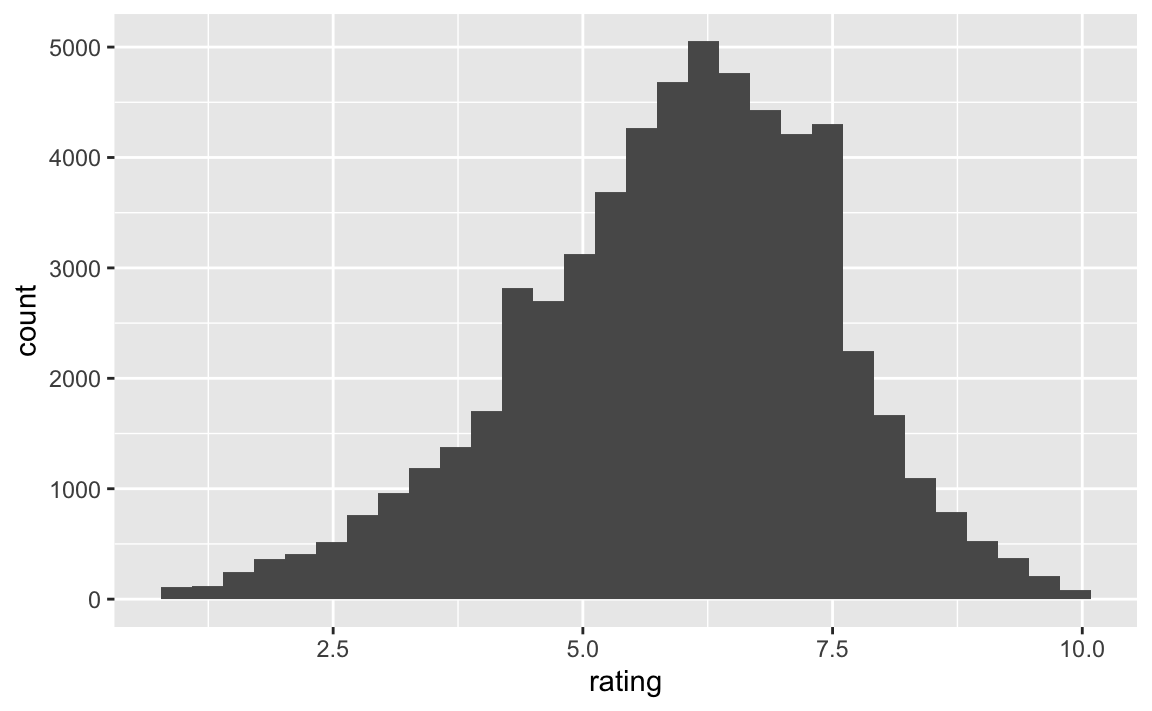
5.4 Distribution of the predictors
movies %>%
  mutate(across(where(is.integer), as.numeric)) %>%  # Integervariable als numerisch deklarieren
  select(where(is.numeric)) %>%  # alle numerischen Variablen auswählen
  pivot_longer(everything(), names_to = "variable") %>%  # auf langes Format pivotieren
  ggplot(aes(x = value)) +
  geom_histogram() +
  facet_wrap(~ variable, scales = "free")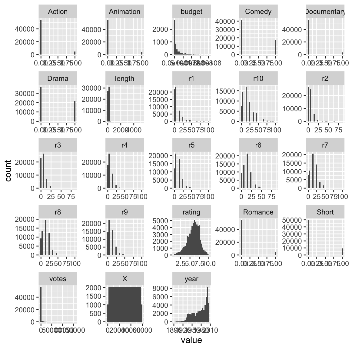
5.5 Transform budget (via logarithm)
movies %>%
  mutate(budget_log10 = log10(budget)) -> movies2
Remove the original variable:
movies2 %>%
  select(budget_log10, everything()) %>%   # "budget_log10" als erste Spalte
  select(-budget) -> movies2
There were some 0 (zero) values in the data set. Taking the logarithm of zero leads to doom. Let’s repair that:
movies2 %>%
  filter(!is.nan(budget_log10)) %>%
  filter(!is.infinite(budget_log10)) -> movies2a
5.6 ggscatterstats
Let’s try this
movies2a %>%
  ggscatterstats(x = budget_log10, y = rating)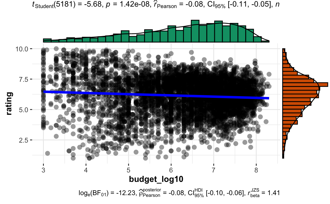
Hier findet sich weitere Erklärung zu diesem Diagramm.
5.7 Pivot data set
movies2a %>%
  select(budget_log10, rating, Action:Short) %>%
  pivot_longer(cols = Action:Short,
               names_to = "genre") %>%
  filter(value == 1) -> movies2_long
And plot it:
movies2_long %>%
  ggplot() +
  aes(x = budget_log10, y = rating) +
  geom_bin2d() +
  facet_wrap(~ genre) +
  geom_smooth() +
  scale_fill_viridis_c()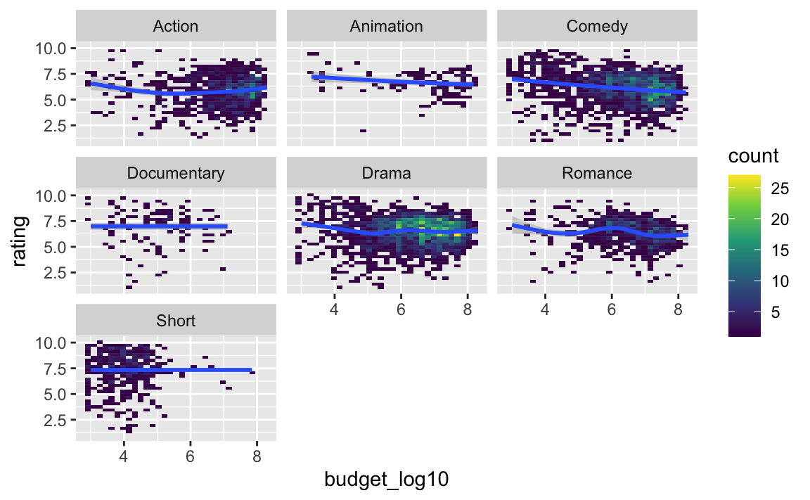
5.8 Drop unused variables
Let’s keep things simple and drop some variables.
movies2a %>%
  select(-c(title, r1:r10, mpaa)) -> movies2a
5.9 Drop cases with missing values
movies2a %>%
  drop_na() -> movies2_nona  # "no NA" soll das heißen
How many row remain?
nrow(movies2_nona)  # "no NAs"
#> [1] 5183
That’s unsatisfying. However, for simplicity, let’s stick with that for now.
6 Model 0
m0 <- lm(rating ~ 1, data = movies2_nona)summary(m0)
#>
#> Call:
#> lm(formula = rating ~ 1, data = movies2_nona)
#>
#> Residuals:
#> Min 1Q Median 3Q Max
#> -5.137 -0.937 0.163 1.063 3.863
#>
#> Coefficients:
#> Estimate Std. Error t value Pr(>|t|)
#> (Intercept) 6.13699 0.02144 286.2 <2e-16 ***
#> ---
#> Signif. codes: 0 '***' 0.001 '**' 0.01 '*' 0.05 '.' 0.1 ' ' 1
#>
#> Residual standard error: 1.544 on 5182 degrees of freedomLet’s make that tidy:
tidy(m0)
#> # A tibble: 1 x 5
#>   term        estimate std.error statistic p.value
#>   <chr>          <dbl>     <dbl>     <dbl>   <dbl>
#> 1 (Intercept)     6.14    0.0214      286.       0
Model fit:
glance(m0)
#> # A tibble: 1 x 12
#>   r.squared adj.r.squared sigma statistic p.value    df logLik    AIC    BIC
#>       <dbl>         <dbl> <dbl>     <dbl>   <dbl> <dbl>  <dbl>  <dbl>  <dbl>
#> 1         0             0  1.54        NA      NA    NA -9605. 19213. 19226.
#> # … with 3 more variables: deviance <dbl>, df.residual <int>, nobs <int>
7 Model 1: budget_log10
movies2_nona %>%
  drop_na(budget_log10, rating) %>%
  lm(rating ~ budget_log10, data = .)  -> m1
tidy(m1)
#> # A tibble: 2 x 5
#> term estimate std.error statistic p.value
#> <chr> <dbl> <dbl> <dbl> <dbl>
#> 1 (Intercept) 6.77 0.113 60.0 0
#> 2 budget_log10 -0.101 0.0178 -5.68 0.0000000142Model fit:
glance(m1)
#> # A tibble: 1 x 12
#>   r.squared adj.r.squared sigma statistic     p.value    df logLik    AIC    BIC
#>       <dbl>         <dbl> <dbl>     <dbl>       <dbl> <dbl>  <dbl>  <dbl>  <dbl>
#> 1   0.00619       0.00600  1.54      32.3     1.42e-8     1 -9589. 19183. 19203.
#> # … with 3 more variables: deviance <dbl>, df.residual <int>, nobs <int>
8 Model 2: Adding number of votes
p1 <- movies2_nona %>%
  ggplot(aes(x = votes)) +
  geom_histogram() +
  labs(title = "Datensatz: movies2_train")

p1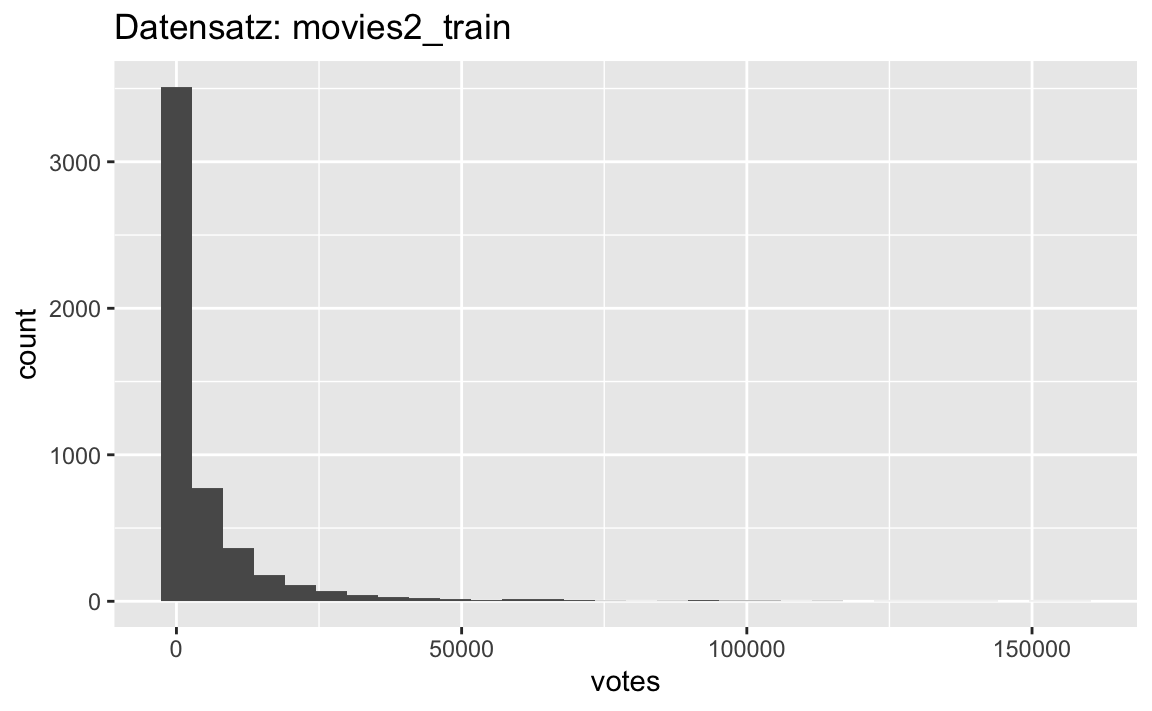
Log-transform votes:
movies2_nona %>%
  mutate(votes_log10 = log10(votes)) %>%
  select(-votes) -> movies3_nona
movies3_nona %>%
lm(rating ~ votes_log10, data = .) -> m2
m2 %>%
tidy()
#> # A tibble: 2 x 5
#> term estimate std.error statistic p.value
#> <chr> <dbl> <dbl> <dbl> <dbl>
#> 1 (Intercept) 5.67 0.0564 100. 0.
#> 2 votes_log10 0.170 0.0191 8.90 7.80e-19
glance(m2)
#> # A tibble: 1 x 12
#> r.squared adj.r.squared sigma statistic p.value df logLik AIC BIC
#> <dbl> <dbl> <dbl> <dbl> <dbl> <dbl> <dbl> <dbl> <dbl>
#> 1 0.0150 0.0149 1.53 79.2 7.80e-19 1 -9565. 19137. 19156.
#> # … with 3 more variables: deviance <dbl>, df.residual <int>, nobs <int>9 Model 3: Number of votes, quadratic
m3 <- lm(rating ~ I(votes_log10^2) + votes_log10, data = movies3_nona)tidy(m3)
#> # A tibble: 3 x 5
#> term estimate std.error statistic p.value
#> <chr> <dbl> <dbl> <dbl> <dbl>
#> 1 (Intercept) 8.24 0.110 74.8 0.
#> 2 I(votes_log10^2) 0.444 0.0167 26.6 8.67e-146
#> 3 votes_log10 -2.18 0.0904 -24.1 3.75e-122glance(m3)
#> # A tibble: 1 x 12
#> r.squared adj.r.squared sigma statistic p.value df logLik AIC BIC
#> <dbl> <dbl> <dbl> <dbl> <dbl> <dbl> <dbl> <dbl> <dbl>
#> 1 0.133 0.133 1.44 398. 2.39e-161 2 -9235. 18477. 18503.
#> # … with 3 more variables: deviance <dbl>, df.residual <int>, nobs <int>movies3_nona %>%
ggplot(aes(x = votes_log10, y = rating)) +
geom_point(alpha = .2) +
geom_smooth(method = "lm", se = FALSE,
formula = y ~ poly(x, 2))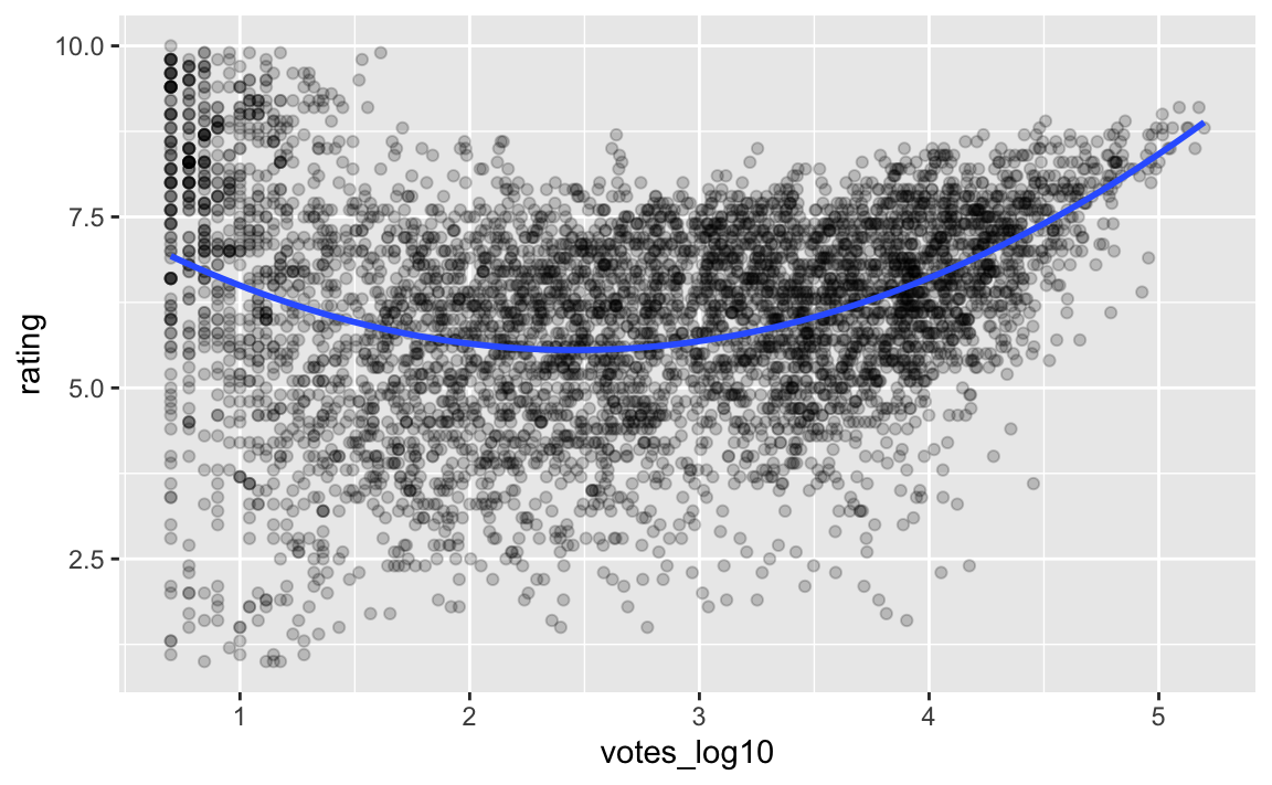
10 Model 4: Number of votes, 3rd degree
movies3_nona %>%
  ggplot(aes(x = votes_log10, y = rating)) +
  geom_point(alpha = .2) +
  geom_smooth(method = "lm", se = FALSE,
                formula = y ~ poly(x, 3))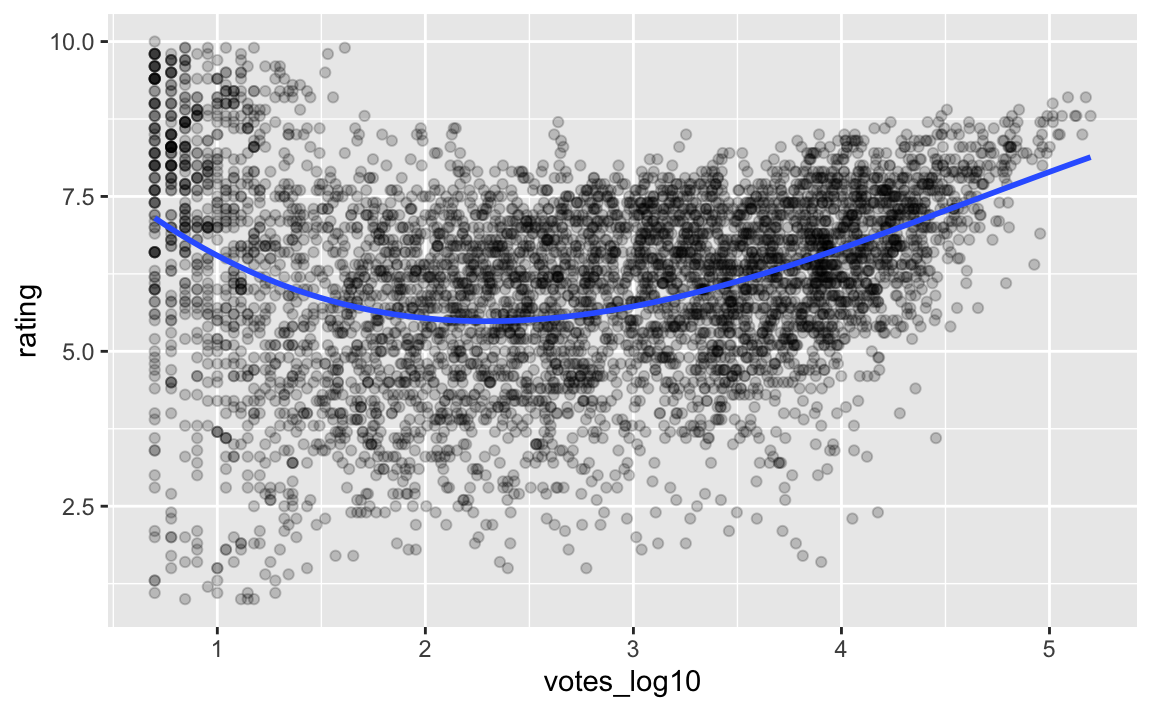
m4 <- lm(rating ~ poly(votes_log10, degree = 3),
         data = movies3_nona)
tidy(m4)
#> # A tibble: 4 x 5
#> term estimate std.error statistic p.value
#> <chr> <dbl> <dbl> <dbl> <dbl>
#> 1 (Intercept) 6.14 0.0199 308. 0.
#> 2 poly(votes_log10, degree = 3)1 13.6 1.43 9.50 2.98e- 21
#> 3 poly(votes_log10, degree = 3)2 38.2 1.43 26.6 1.99e-146
#> 4 poly(votes_log10, degree = 3)3 -7.26 1.43 -5.06 4.27e- 7
glance(m4)
#> # A tibble: 1 x 12
#> r.squared adj.r.squared sigma statistic p.value df logLik AIC BIC
#> <dbl> <dbl> <dbl> <dbl> <dbl> <dbl> <dbl> <dbl> <dbl>
#> 1 0.137 0.137 1.43 275. 1.53e-165 3 -9222. 18454. 18486.
#> # … with 3 more variables: deviance <dbl>, df.residual <int>, nobs <int>11 Model 5: Multiple regression
m5 <- lm(rating ~ votes_log10 + budget_log10, data = movies3_nona)glance(m5)
#> # A tibble: 1 x 12
#> r.squared adj.r.squared sigma statistic p.value df logLik AIC BIC
#> <dbl> <dbl> <dbl> <dbl> <dbl> <dbl> <dbl> <dbl> <dbl>
#> 1 0.0877 0.0874 1.47 249. 5.02e-104 2 -9367. 18741. 18768.
#> # … with 3 more variables: deviance <dbl>, df.residual <int>, nobs <int>12 Model 6: Interaction
m6 <- lm(rating ~ votes_log10 + budget_log10 + votes_log10:budget_log10,
         data = movies3_nona)
13 Model selection: ANOVA
anova(m0,  m2, m3, m4)
#> Analysis of Variance Table
#>
#> Model 1: rating ~ 1
#> Model 2: rating ~ votes_log10
#> Model 3: rating ~ I(votes_log10^2) + votes_log10
#> Model 4: rating ~ poly(votes_log10, degree = 3)
#>   Res.Df   RSS Df Sum of Sq       F    Pr(>F)
#> 1   5182 12351
#> 2   5181 12165  1    185.86  90.341 < 2.2e-16 ***
#> 3   5180 10707  1   1457.68 708.550 < 2.2e-16 ***
#> 4   5179 10655  1     52.74  25.636 4.265e-07 ***
#> ---
#> Signif. codes:  0 '***' 0.001 '**' 0.01 '*' 0.05 '.' 0.1 ' ' 1
This test assesses:
\[F =\frac{(TSS-RSS)/p}{RSS/(n-p-1)}\]
glance(m6)
#> # A tibble: 1 x 12
#>   r.squared adj.r.squared sigma statistic   p.value    df logLik    AIC    BIC
#>       <dbl>         <dbl> <dbl>     <dbl>     <dbl> <dbl>  <dbl>  <dbl>  <dbl>
#> 1     0.117         0.117  1.45      230. 6.88e-140     3 -9281. 18572. 18605.
#> # … with 3 more variables: deviance <dbl>, df.residual <int>, nobs <int>
14 Regression diagnostics: testing the assumptions
Let’s pick a model and visualize some diagnostics.
ggplot2::autoplot(m4) + theme_minimal()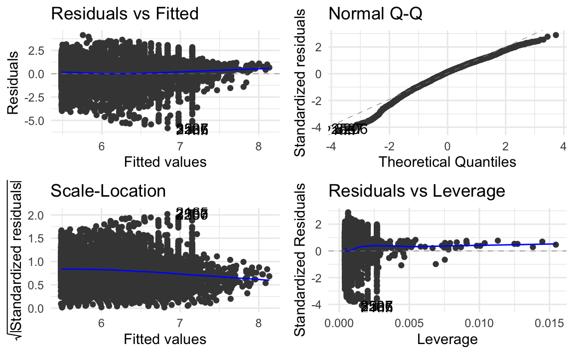
15 Reproducibility
#> ─ Session info ───────────────────────────────────────────────────────────────────────────────────────────────────────
#>  setting  value
#>  version  R version 4.0.2 (2020-06-22)
#>  os       macOS  10.16
#>  system   x86_64, darwin17.0
#>  ui       X11
#>  language (EN)
#>  collate  en_US.UTF-8
#>  ctype    en_US.UTF-8
#>  tz       Europe/Berlin
#>  date     2021-02-24
#>
#> ─ Packages ───────────────────────────────────────────────────────────────────────────────────────────────────────────
#>  package     * version     date       lib source
#>  assertthat    0.2.1       2019-03-21 [1] CRAN (R 4.0.0)
#>  backports     1.2.1       2020-12-09 [1] CRAN (R 4.0.2)
#>  blogdown      1.1         2021-01-19 [1] CRAN (R 4.0.2)
#>  bookdown      0.21.6      2021-02-02 [1] Github (rstudio/bookdown@6c7346a)
#>  broom         0.7.5       2021-02-19 [1] CRAN (R 4.0.2)
#>  bslib         0.2.4.9000  2021-02-02 [1] Github (rstudio/bslib@b3cd7a9)
#>  cachem        1.0.4       2021-02-13 [1] CRAN (R 4.0.2)
#>  callr         3.5.1       2020-10-13 [1] CRAN (R 4.0.2)
#>  cellranger    1.1.0       2016-07-27 [1] CRAN (R 4.0.0)
#>  cli           2.3.1       2021-02-23 [1] CRAN (R 4.0.2)
#>  codetools     0.2-16      2018-12-24 [2] CRAN (R 4.0.2)
#>  colorspace    2.0-0       2020-11-11 [1] CRAN (R 4.0.2)
#>  crayon        1.4.1       2021-02-08 [1] CRAN (R 4.0.2)
#>  DBI           1.1.1       2021-01-15 [1] CRAN (R 4.0.2)
#>  dbplyr        2.1.0       2021-02-03 [1] CRAN (R 4.0.2)
#>  debugme       1.1.0       2017-10-22 [1] CRAN (R 4.0.0)
#>  desc          1.2.0       2018-05-01 [1] CRAN (R 4.0.0)
#>  devtools      2.3.2       2020-09-18 [1] CRAN (R 4.0.2)
#>  digest        0.6.27      2020-10-24 [1] CRAN (R 4.0.2)
#>  dplyr       * 1.0.4       2021-02-02 [1] CRAN (R 4.0.2)
#>  ellipsis      0.3.1       2020-05-15 [1] CRAN (R 4.0.0)
#>  evaluate      0.14        2019-05-28 [1] CRAN (R 4.0.0)
#>  fansi         0.4.2       2021-01-15 [1] CRAN (R 4.0.2)
#>  fastmap       1.1.0       2021-01-25 [1] CRAN (R 4.0.2)
#>  forcats     * 0.5.1       2021-01-27 [1] CRAN (R 4.0.2)
#>  fs            1.5.0       2020-07-31 [1] CRAN (R 4.0.2)
#>  generics      0.1.0       2020-10-31 [1] CRAN (R 4.0.2)
#>  ggplot2     * 3.3.3       2020-12-30 [1] CRAN (R 4.0.2)
#>  glue          1.4.2       2020-08-27 [1] CRAN (R 4.0.2)
#>  gtable        0.3.0       2019-03-25 [1] CRAN (R 4.0.0)
#>  haven         2.3.1       2020-06-01 [1] CRAN (R 4.0.0)
#>  hms           1.0.0       2021-01-13 [1] CRAN (R 4.0.2)
#>  htmltools     0.5.1.1     2021-01-22 [1] CRAN (R 4.0.2)
#>  httr          1.4.2       2020-07-20 [1] CRAN (R 4.0.2)
#>  jquerylib     0.1.3       2020-12-17 [1] CRAN (R 4.0.2)
#>  jsonlite      1.7.2       2020-12-09 [1] CRAN (R 4.0.2)
#>  knitr         1.31        2021-01-27 [1] CRAN (R 4.0.2)
#>  lifecycle     1.0.0       2021-02-15 [1] CRAN (R 4.0.2)
#>  lubridate     1.7.9.2     2020-11-13 [1] CRAN (R 4.0.2)
#>  magrittr      2.0.1       2020-11-17 [1] CRAN (R 4.0.2)
#>  memoise       2.0.0       2021-01-26 [1] CRAN (R 4.0.2)
#>  modelr        0.1.8       2020-05-19 [1] CRAN (R 4.0.0)
#>  munsell       0.5.0       2018-06-12 [1] CRAN (R 4.0.0)
#>  pillar        1.5.0       2021-02-22 [1] CRAN (R 4.0.2)
#>  pkgbuild      1.2.0       2020-12-15 [1] CRAN (R 4.0.2)
#>  pkgconfig     2.0.3       2019-09-22 [1] CRAN (R 4.0.0)
#>  pkgload       1.2.0       2021-02-23 [1] CRAN (R 4.0.2)
#>  prettyunits   1.1.1       2020-01-24 [1] CRAN (R 4.0.0)
#>  processx      3.4.5       2020-11-30 [1] CRAN (R 4.0.2)
#>  ps            1.5.0       2020-12-05 [1] CRAN (R 4.0.2)
#>  purrr       * 0.3.4       2020-04-17 [1] CRAN (R 4.0.0)
#>  R6            2.5.0       2020-10-28 [1] CRAN (R 4.0.2)
#>  Rcpp          1.0.6       2021-01-15 [1] CRAN (R 4.0.2)
#>  readr       * 1.4.0       2020-10-05 [1] CRAN (R 4.0.2)
#>  readxl        1.3.1       2019-03-13 [1] CRAN (R 4.0.0)
#>  remotes       2.2.0       2020-07-21 [1] CRAN (R 4.0.2)
#>  reprex        1.0.0       2021-01-27 [1] CRAN (R 4.0.2)
#>  rlang         0.4.10      2020-12-30 [1] CRAN (R 4.0.2)
#>  rmarkdown     2.7         2021-02-19 [1] CRAN (R 4.0.2)
#>  rprojroot     2.0.2       2020-11-15 [1] CRAN (R 4.0.2)
#>  rstudioapi    0.13.0-9000 2021-02-11 [1] Github (rstudio/rstudioapi@9d21f50)
#>  rvest         0.3.6       2020-07-25 [1] CRAN (R 4.0.2)
#>  sass          0.3.1       2021-01-24 [1] CRAN (R 4.0.2)
#>  scales        1.1.1       2020-05-11 [1] CRAN (R 4.0.0)
#>  sessioninfo   1.1.1       2018-11-05 [1] CRAN (R 4.0.0)
#>  stringi       1.5.3       2020-09-09 [1] CRAN (R 4.0.2)
#>  stringr     * 1.4.0       2019-02-10 [1] CRAN (R 4.0.0)
#>  testthat      3.0.2       2021-02-14 [1] CRAN (R 4.0.2)
#>  tibble      * 3.0.6       2021-01-29 [1] CRAN (R 4.0.2)
#>  tidyr       * 1.1.2       2020-08-27 [1] CRAN (R 4.0.2)
#>  tidyselect    1.1.0       2020-05-11 [1] CRAN (R 4.0.0)
#>  tidyverse   * 1.3.0       2019-11-21 [1] CRAN (R 4.0.0)
#>  usethis       2.0.1       2021-02-10 [1] CRAN (R 4.0.2)
#>  utf8          1.1.4       2018-05-24 [1] CRAN (R 4.0.0)
#>  vctrs         0.3.6       2020-12-17 [1] CRAN (R 4.0.2)
#>  withr         2.4.1       2021-01-26 [1] CRAN (R 4.0.2)
#>  xfun          0.21        2021-02-10 [1] CRAN (R 4.0.2)
#>  xml2          1.3.2       2020-04-23 [1] CRAN (R 4.0.0)
#>  yaml          2.2.1       2020-02-01 [1] CRAN (R 4.0.0)
#>
#> [1] /Users/sebastiansaueruser/Rlibs
#> [2] /Library/Frameworks/R.framework/Versions/4.0/Resources/library