1 Motivation
Being a teacher (in some part of my life), I conducted a prediction contest. Students had to predict a bunch of values as precisely as possible. That’s the sort of stuff data scientist do (or are said to do). As far as I am concerned, I was looking at a convenient way of grading the prediction data. Here’s an attempt.
I’m sorry that post is not fully reproducible. The reason is a privacy rights of my students and that I do not want to fully undisclosure the data set I used, because I might use it for upcoming student cohorts. Teachers: Feel free to contact me if you like to know more about the data set.
2 Setup
library(tidyverse)
library(testthat)
library(data.table)
library(glue)
library(here)
library(skimr)
Use ?data.table etc. for help on the packages.
3 Helper functions
3.1 Function to parse data
One trouble is that the CSV files I expected can be in different formats: standard CSV, CSV2 (semicolon delimiter, comma decimal). That’s why we need to come up with a more general data parsing function. Unfortunately, and to my suprise, I found no existing funtion that was able to deal with that matter (no, even fread did not).
try_readcsv <- function(file, verbose = FALSE) {

  # import csv file:
  x <- data.table::fread(file, header = TRUE)

  # if more than 2 columns, only select first and last one:
  if (ncol(x) > 2) {
    x <- x %>%
      select(1, last_col())
  }

  # stop if only one column:
  if (ncol(x) == 1) stop("Only 1 column! There should be (at least) two: ID and predictions.")

  # set names:
  names(x) <- c("id", "pred")

  # replace commas with dots to deal with German locale:
  x <-
    x %>%
    mutate(across(where(is.character),
                  .fns = ~ str_replace_all(.,
                                           pattern = ",",
                                           replacement = ".")))

  # check how many columns where found in each CSV file:
  if (verbose == TRUE) {print("Ncol: "); print(ncol(x))}
  return(x)

}
3.2 Function to compute \(R^2\)
r2 <- function(predicted, observed) {

  rss <- sum((predicted - observed) ^ 2)  ## residual sum of squares
  tss <- sum((observed - mean(observed)) ^ 2)  ## total sum of squares
  rsq <- 1 - rss/tss

  return(rsq)

}
3.3 Function to compute \(MSE\)
Mean Squared Error
mse <- function(predicted, observed) {

  mse <- mean((predicted - observed) ^ 2)  ## mean residual sum of squares

  return(mse)

}
3.4 Function to compute generalized error function
gen_error <- function(predicted, observed, degree = 1) {

  generr <- mean(abs(predicted - observed) ^ degree)  ## mean residual sum of absolute errors to the `degree` power

  return(generr)

}
4 Import solution (true) data (ie., solution)
Define solution file name, and check whether this file name exists:
solution_filename <- paste0("/Users/sebastiansaueruser/Google Drive/Lehre/Lehre_AKTUELL/2020-WiSe/WisMeth/Prognose-Wettbewerb/Prognose-Material/Material-nur-fuer-Lehrende/test_df_teacher.csv")

stopifnot(file.exists(solution_filename))
Import the solution data:
test_df_teacher <- read_csv(solution_filename)

test_df_teacher <-
  test_df_teacher %>%
  mutate(id = row_number()) %>%
  select(id, pay)
5 Parse the data
Get the list of existing files.
Here’s the project path; in your case it will be different.
proj_path <- "/Users/sebastiansaueruser/Google Drive/Lehre/Lehre_AKTUELL/2020-WiSe/WisMeth/Prognose-Wettbewerb/Prognose-Material"subm_path <- paste0(proj_path, "/Submissions/")
submissions <- list.files(path = subm_path,
pattern = "\\.csv$",
recursive = TRUE,
full.names = TRUE)Here is the list of CSV files:
submissions %>%
  head()
#> [1] "/Users/sebastiansaueruser/Google Drive/Lehre/Lehre_AKTUELL/2020-WiSe/WisMeth/Prognose-Wettbewerb/Prognose-Material/Submissions//64d4faba5afe920efbf0001812299853.csv"
#> [2] "/Users/sebastiansaueruser/Google Drive/Lehre/Lehre_AKTUELL/2020-WiSe/WisMeth/Prognose-Wettbewerb/Prognose-Material/Submissions//9c31e89af1b4b1bc67c639708f5b5fa3.csv"
No worries. That are anonymized data files.
The length of this vector should match the number of students (or student teams) we expect:
length(submissions)
#> [1] 2
6 Build master data frame
We build a list data frame for a tidyverse style data manipulation.
6.1 List df where each submission is one row
subm_df <-
  # create column file submission names:
  tibble(filepath = submissions) %>%

  # cut the path away, leave only the file name:
  mutate(filename = str_extract(filepath, "/[^/]*.csv$")) %>%

  # create list column with submission data:
  mutate(subm_data = purrr::map(.x = filepath,
                                .f = ~ try_readcsv(.x))) %>%

  # unnest the columns of the list column:
  unnest_wider(subm_data)
See:
subm_df
#> # A tibble: 2 x 4
#>   filepath                                filename              id       pred
#>   <chr>                                   <chr>                 <list>   <list>
#> 1 /Users/sebastiansaueruser/Google Drive… /64d4faba5afe920efbf… <int [3… <chr […
#> 2 /Users/sebastiansaueruser/Google Drive… /9c31e89af1b4b1bc67c… <int [3… <chr […
Check if all values of pred are of type character:
map_chr(subm_df$pred, class)
#> [1] "character" "character"
Which is the case. This is an artifact of data import; some CSV files had a German decimal delimiter (dot) whereas others used the standard (comma). So, a robust strategy is to parse those strange numbers all as characters. Then replace the delimiting commas with dots. Then transform to numeric. See the import function above for details.
6.2 Change character to numeric
We need to convert pred to numeric:
subm_df2 <-
  subm_df %>%
  # render character into numeric (still a list column, hence we need the `map`):
  mutate(pred_num = map(pred, as.numeric))
Check if all values still are of type character:
subm_df2$pred_num %>%
  map_chr(class)  %>%
  unique()
#> [1] "numeric"
Nope. Numeric, as it should be.
More programmatically:
subm_df2$pred_num %>%
  map_chr(class)  %>%
  unique() %>%
  length() %>%
  expect_equal(1)
6.3 Add observed (true) values
subm_df3 <-
  subm_df2 %>%
  # add y-value (to be predicted), again a list column:
  mutate(observed = list(test_df_teacher$pay))
See:
head(subm_df3)
#> # A tibble: 2 x 6
#>   filepath                    filename         id      pred    pred_num observed
#>   <chr>                       <chr>            <list>  <list>  <list>   <list>
#> 1 /Users/sebastiansaueruser/… /64d4faba5afe92… <int [… <chr [… <dbl [3… <dbl [3…
#> 2 /Users/sebastiansaueruser/… /9c31e89af1b4b1… <int [… <chr [… <dbl [3… <dbl [3…
6.4 Check lengths of submissions
subm_df3$id %>%
  map_dbl(length) %>%
  unique()
#> [1] 300
subm_df3$id %>%
map_dbl(length) %>%
unique() %>%
length() %>%
expect_equal(1)Each submission should consist of 300 entries in this example.
7 Compute accuracy (\(R^2\) etc.)
subm_df4 <-
  subm_df3 %>%
  mutate(r2 = map2(.x = pred_num,
                     .y = observed,
                     .f = ~ r2(.x, .y)),
         mse = map2(.x = pred_num,
                     .y = observed,
                     .f = ~ mse(.x, .y)),
         mae = map2(.x = pred_num,
                     .y = observed,
                     .f = ~ gen_error(.x, .y))) %>%
  unnest(r2)
See:
subm_df4 %>%
  glimpse()
#> Rows: 2
#> Columns: 9
#> $ filepath <chr> "/Users/sebastiansaueruser/Google Drive/Lehre/Lehre_AKTUELL/…
#> $ filename <chr> "/64d4faba5afe920efbf0001812299853.csv", "/9c31e89af1b4b1bc6…
#> $ id       <list> [<1, 2, 3, 4, 5, 6, 7, 8, 9, 10, 11, 12, 13, 14, 15, 16, 17…
#> $ pred     <list> [<"102622.898614099", "110032.651526331", "97047.9425798611…
#> $ pred_num <list> [<102622.90, 110032.65, 97047.94, 60826.89, 168182.88, 1562…
#> $ observed <list> [<91336, 112286, 77536, 69872, 156896, 151509, 78267, 12535…
#> $ r2       <dbl> 0.8287524, 0.8280914
#> $ mse      <list> [107043353, 107456477]
#> $ mae      <list> [8392.041, 8453.271]
7.1 Check distribution of \(R^2\)
subm_df4 %>%
  filter(between(r2,0, 1)) %>%
  summarise(r2_mean = mean(r2),
            r2_sd = sd(r2),
            r2_med = median(r2),
            r2_iqr = IQR(r2),
            r2_min = min(r2),
            r2_max = max(r2))
#> # A tibble: 1 x 6
#>   r2_mean    r2_sd r2_med   r2_iqr r2_min r2_max
#>     <dbl>    <dbl>  <dbl>    <dbl>  <dbl>  <dbl>
#> 1   0.828 0.000467  0.828 0.000330  0.828  0.829
subm_df4 %>%
filter(between(r2, 0, 1)) %>%
ggplot(aes(x = r2)) +
geom_histogram()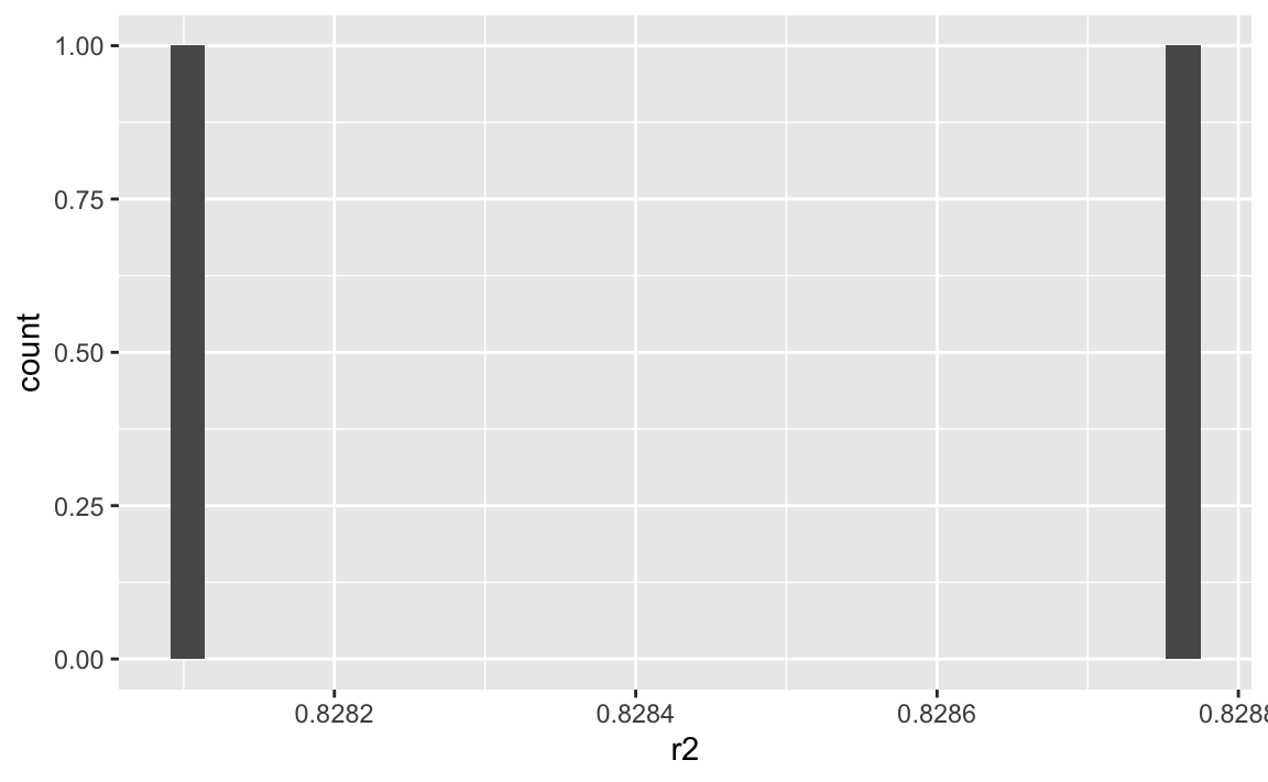
7.2 Number of distinct values for \(R^2\)
length(unique(subm_df4$r2))
#> [1] 2
8 Grading
8.1 Note-4.0 model
note4_r2 <- 0.018.2 Note-1.0 model
note1_r2 <- 0.838.3 Grades in sequence
There are 10 grades (from 4.0 to 1.0), plus the 5 (fail), plus the “supra-best” (only to define the maximum threshold), giving 12 grades in total.
grades_df <-
  tibble(thresholds = c(0,
                        seq(from = 0.01, to = 0.83,
                            length.out = 9), .85, 1),
         thresholds2 = c(0,
                         seq(from = .51, to = 1,
                             length.out = 11)),
         grades = c(5, 4, 3.7, 3.3, 3.0, 2.7, 2.3, 2, 1.7, 1.3, 1, .7)) %>%
  mutate(id = nrow(.):1)
grades_df
#> # A tibble: 12 x 4
#>    thresholds thresholds2 grades    id
#>         <dbl>       <dbl>  <dbl> <int>
#>  1      0           0        5      12
#>  2      0.01        0.51     4      11
#>  3      0.112       0.559    3.7    10
#>  4      0.215       0.608    3.3     9
#>  5      0.318       0.657    3       8
#>  6      0.42        0.706    2.7     7
#>  7      0.522       0.755    2.3     6
#>  8      0.625       0.804    2       5
#>  9      0.727       0.853    1.7     4
#> 10      0.83        0.902    1.3     3
#> 11      0.85        0.951    1       2
#> 12      1           1        0.7     1
8.4 Map grades to individual \(R^2\) values of the students
subm_df5 <-
  subm_df4 %>%
  mutate(grade_id = map_dbl(r2,
                         .f = ~ {`>`(grades_df$thresholds, .x) %>% sum()} )) %>%
  left_join(grades_df %>% select(-c(thresholds, thresholds2)),
            by = c("grade_id" = "id"))
8.5 Grade distribution
subm_df5 %>%
  select(grades) %>%
skim()| Name | Piped data |
| Number of rows | 2 |
| Number of columns | 1 |
| _______________________ | |
| Column type frequency: | |
| numeric | 1 |
| ________________________ | |
| Group variables | None |
Variable type: numeric
| skim_variable | n_missing | complete_rate | mean | sd | p0 | p25 | p50 | p75 | p100 | hist |
|---|---|---|---|---|---|---|---|---|---|---|
| grades | 0 | 1 | 1.3 | 0 | 1.3 | 1.3 | 1.3 | 1.3 | 1.3 | ▁▁▇▁▁ |
9 Reproducibility
#> ─ Session info ───────────────────────────────────────────────────────────────────────────────────────────────────────
#>  setting  value
#>  version  R version 4.0.2 (2020-06-22)
#>  os       macOS  10.16
#>  system   x86_64, darwin17.0
#>  ui       X11
#>  language (EN)
#>  collate  en_US.UTF-8
#>  ctype    en_US.UTF-8
#>  tz       Europe/Berlin
#>  date     2021-01-20
#>
#> ─ Packages ───────────────────────────────────────────────────────────────────────────────────────────────────────────
#>  package     * version     date       lib source
#>  assertthat    0.2.1       2019-03-21 [1] CRAN (R 4.0.0)
#>  backports     1.2.0       2020-11-02 [1] CRAN (R 4.0.2)
#>  blogdown      0.21        2020-10-11 [1] CRAN (R 4.0.2)
#>  bookdown      0.21        2020-10-13 [1] CRAN (R 4.0.2)
#>  broom         0.7.2       2020-10-20 [1] CRAN (R 4.0.2)
#>  callr         3.5.1       2020-10-13 [1] CRAN (R 4.0.2)
#>  cellranger    1.1.0       2016-07-27 [1] CRAN (R 4.0.0)
#>  cli           2.2.0       2020-11-20 [1] CRAN (R 4.0.2)
#>  codetools     0.2-16      2018-12-24 [2] CRAN (R 4.0.2)
#>  colorspace    2.0-0       2020-11-11 [1] CRAN (R 4.0.2)
#>  crayon        1.3.4       2017-09-16 [1] CRAN (R 4.0.0)
#>  DBI           1.1.0       2019-12-15 [1] CRAN (R 4.0.0)
#>  dbplyr        2.0.0       2020-11-03 [1] CRAN (R 4.0.2)
#>  desc          1.2.0       2018-05-01 [1] CRAN (R 4.0.0)
#>  devtools      2.3.2       2020-09-18 [1] CRAN (R 4.0.2)
#>  digest        0.6.27      2020-10-24 [1] CRAN (R 4.0.2)
#>  dplyr       * 1.0.2       2020-08-18 [1] CRAN (R 4.0.2)
#>  ellipsis      0.3.1       2020-05-15 [1] CRAN (R 4.0.0)
#>  evaluate      0.14        2019-05-28 [1] CRAN (R 4.0.0)
#>  fansi         0.4.1       2020-01-08 [1] CRAN (R 4.0.0)
#>  forcats     * 0.5.0       2020-03-01 [1] CRAN (R 4.0.0)
#>  fs            1.5.0       2020-07-31 [1] CRAN (R 4.0.2)
#>  generics      0.1.0       2020-10-31 [1] CRAN (R 4.0.2)
#>  ggplot2     * 3.3.2       2020-06-19 [1] CRAN (R 4.0.0)
#>  glue          1.4.2       2020-08-27 [1] CRAN (R 4.0.2)
#>  gtable        0.3.0       2019-03-25 [1] CRAN (R 4.0.0)
#>  haven         2.3.1       2020-06-01 [1] CRAN (R 4.0.0)
#>  hms           0.5.3       2020-01-08 [1] CRAN (R 4.0.0)
#>  htmltools     0.5.0       2020-06-16 [1] CRAN (R 4.0.0)
#>  httr          1.4.2       2020-07-20 [1] CRAN (R 4.0.2)
#>  jsonlite      1.7.1       2020-09-07 [1] CRAN (R 4.0.2)
#>  knitr         1.30        2020-09-22 [1] CRAN (R 4.0.2)
#>  lifecycle     0.2.0       2020-03-06 [1] CRAN (R 4.0.0)
#>  lubridate     1.7.9.2     2020-11-13 [1] CRAN (R 4.0.2)
#>  magrittr      2.0.1       2020-11-17 [1] CRAN (R 4.0.2)
#>  memoise       1.1.0       2017-04-21 [1] CRAN (R 4.0.0)
#>  modelr        0.1.8       2020-05-19 [1] CRAN (R 4.0.0)
#>  munsell       0.5.0       2018-06-12 [1] CRAN (R 4.0.0)
#>  pillar        1.4.7       2020-11-20 [1] CRAN (R 4.0.2)
#>  pkgbuild      1.1.0       2020-07-13 [1] CRAN (R 4.0.2)
#>  pkgconfig     2.0.3       2019-09-22 [1] CRAN (R 4.0.0)
#>  pkgload       1.1.0       2020-05-29 [1] CRAN (R 4.0.0)
#>  prettyunits   1.1.1       2020-01-24 [1] CRAN (R 4.0.0)
#>  processx      3.4.5       2020-11-30 [1] CRAN (R 4.0.2)
#>  ps            1.4.0       2020-10-07 [1] CRAN (R 4.0.2)
#>  purrr       * 0.3.4       2020-04-17 [1] CRAN (R 4.0.0)
#>  R6            2.5.0       2020-10-28 [1] CRAN (R 4.0.2)
#>  Rcpp          1.0.5       2020-07-06 [1] CRAN (R 4.0.2)
#>  readr       * 1.4.0       2020-10-05 [1] CRAN (R 4.0.2)
#>  readxl        1.3.1       2019-03-13 [1] CRAN (R 4.0.0)
#>  remotes       2.2.0       2020-07-21 [1] CRAN (R 4.0.2)
#>  reprex        0.3.0       2019-05-16 [1] CRAN (R 4.0.0)
#>  rlang         0.4.9       2020-11-26 [1] CRAN (R 4.0.2)
#>  rmarkdown     2.5         2020-10-21 [1] CRAN (R 4.0.2)
#>  rprojroot     2.0.2       2020-11-15 [1] CRAN (R 4.0.2)
#>  rstudioapi    0.13.0-9000 2020-12-09 [1] Github (rstudio/rstudioapi@4baeb39)
#>  rvest         0.3.6       2020-07-25 [1] CRAN (R 4.0.2)
#>  scales        1.1.1       2020-05-11 [1] CRAN (R 4.0.0)
#>  sessioninfo   1.1.1       2018-11-05 [1] CRAN (R 4.0.0)
#>  stringi       1.5.3       2020-09-09 [1] CRAN (R 4.0.2)
#>  stringr     * 1.4.0       2019-02-10 [1] CRAN (R 4.0.0)
#>  testthat      3.0.0       2020-10-31 [1] CRAN (R 4.0.2)
#>  tibble      * 3.0.4       2020-10-12 [1] CRAN (R 4.0.2)
#>  tidyr       * 1.1.2       2020-08-27 [1] CRAN (R 4.0.2)
#>  tidyselect    1.1.0       2020-05-11 [1] CRAN (R 4.0.0)
#>  tidyverse   * 1.3.0       2019-11-21 [1] CRAN (R 4.0.0)
#>  usethis       1.6.3       2020-09-17 [1] CRAN (R 4.0.2)
#>  vctrs         0.3.5       2020-11-17 [1] CRAN (R 4.0.2)
#>  withr         2.3.0       2020-09-22 [1] CRAN (R 4.0.2)
#>  xfun          0.19        2020-10-30 [1] CRAN (R 4.0.2)
#>  xml2          1.3.2       2020-04-23 [1] CRAN (R 4.0.0)
#>  yaml          2.2.1       2020-02-01 [1] CRAN (R 4.0.0)
#>
#> [1] /Users/sebastiansaueruser/Rlibs
#> [2] /Library/Frameworks/R.framework/Versions/4.0/Resources/library