UPDATE 2020-11-30 based on discussion with Norman Markgraf, see disqus below.
A story about data
Say we have a decent sample of , and we would like to compute a standard, plain vanilla confidence interval (95% CI).
For the sake of having a story, assume you are the boss of the NYC airports and you are investigating the 2013 “typical” arrival delays.
OK, here we go.
Get the sample:
set.seed(42)
flights_sample <- sample_n(drop_na(flights, arr_delay),
                           size = 30)
Note that it does not matter which particular sample we draw. Our argument is: Given some sample, what can we derive for a confidence interval?
Compute the discriptives:
favstats(~ arr_delay,
         data = flights_sample)
#>  min Q1 median   Q3 max mean       sd  n missing
#>  -26 -6      0 7.25  39  1.5 14.91528 30       0
In more tidyverse terms:
flights_sample %>%
  drop_na(arr_delay) %>%
  summarise(delay_avg = mean(arr_delay),
            delay_sd = sd(arr_delay)) -> flights_summary

flights_summary
#> # A tibble: 1 x 2
#>   delay_avg delay_sd
#>       <dbl>    <dbl>
#> 1       1.5     14.9
Wonderful. Now walk on to the CI.
Confidence interval around the mean
flights_summary %>%
  mutate(delay_n = nrow(flights_sample),
         delay_sem = delay_sd / sqrt(delay_n),
         delay_95ci_lower = delay_avg - 1.96 * delay_sem,
         delay_95ci_upper = delay_avg + 1.96 * delay_sem) -> flights_summary

flights_summary
#> # A tibble: 1 x 6
#>   delay_avg delay_sd delay_n delay_sem delay_95ci_lower delay_95ci_upper
#>       <dbl>    <dbl>   <int>     <dbl>            <dbl>            <dbl>
#> 1       1.5     14.9      30      2.72            -3.84             6.84
Plot the CI
Define some constants for the sake of brevity:
flights_avg <- flights_summary$delay_avg
flights_sem <- flights_summary$delay_sem
ggplot(data.frame(x = c(-7,10)), aes(x = x)) +
stat_function(fun = dnorm, n = 1000,
args = c(mean = flights_avg,
sd = flights_sem)) +
labs(title = "Distribution based confidence interval",
subtitle = paste0("Mean: ",
round(flights_avg, 2),
",\nSE: ", round(flights_sem, 2)),
caption = "Vertical dashed bars indicate the confidence interval borders") +
geom_vline(xintercept = c(flights_avg + 1.96 * flights_sem,
flights_avg - 1.96 * flights_sem),
color = "blue", linetype = "dashed")
CI using simulation
boot1 <- do(10000) * mean(~ arr_delay, na.rm = T,
                         data = resample(flights_sample))
boot_mean <- mean(~mean, data = boot1)
boot_mean
#> [1] 1.508767
boot_sd = sd(~ mean, data = boot1)
boot_sd
#> [1] 2.741748ggplot(data.frame(x = c(-7,10)), aes(x = x)) +
stat_function(fun = dnorm, n = 1000,
args = c(mean = boot_mean,
sd = boot_sd)) +
labs(subtitle = paste0("Mean: ", round(boot_mean, 2),
",\nSE: ",
round(boot_sd, 2)),
title = "Distribution based CI with boostrapped SD",
caption = "Vertical dashed bars indicate the confidence interval borders") +
geom_vline(xintercept = c(boot_mean + 2* boot_sd,
boot_mean - 2* boot_sd),
color = "blue", linetype = "dashed")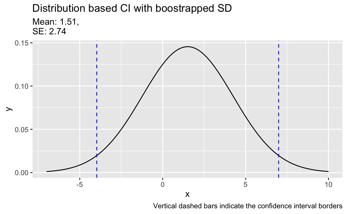
And for the sake of completeness, here are the limits of the boostrapped CI:
confint(boot1)
#>   name   lower  upper level     method estimate
#> 1 mean -3.6675 6.9675  0.95 percentile      1.5
And here’s the pure non-parametric bootstrap interval:
ggplot(boot1, aes(x = mean)) +
  geom_density() +
  labs(subtitle = paste0("Mean: ", round(boot_mean, 2),
                                   ",\nSE: ", round(boot_mean, 2)),
       title = "Simulation based (bootstrap) CI",
        caption = "Vertical dashed bars indicate the confidence interval borders") +
  geom_vline(aes(xintercept = confint(boot1)$lower[1]),
             color = "blue", linetype = "dashed") +
  geom_vline(aes(xintercept = confint(boot1)$upper[1]),
             color = "blue", linetype = "dashed")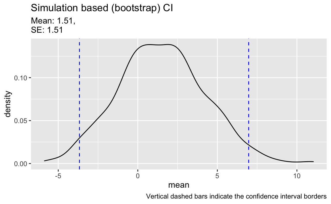
Myth time
Some one claims:
“A CI is the interval where 95% of all possible sample means fall into”.
Let’s check that.
Draw many samples from the population
Taking flights as the population, let’s draw many samples from it, say 100.
flights_many_samples <- flights %>%
  select(arr_delay) %>%
  drop_na(arr_delay) %>%
  sample_n(100*100) %>%
  mutate(sample_id = rep(1:100, times = 100))

flights_many_samples
#> # A tibble: 10,000 x 2
#>    arr_delay sample_id
#>        <dbl>     <int>
#>  1        -3         1
#>  2       -12         2
#>  3         5         3
#>  4       -12         4
#>  5       -12         5
#>  6        88         6
#>  7        17         7
#>  8        -5         8
#>  9        -4         9
#> 10        -6        10
#> # … with 9,990 more rows
flights_many_samples %>%
group_by(sample_id) %>%
summarise(delay_sample_avg = mean(arr_delay)) -> flights_many_samples_summary
flights_many_samples_summary
#> # A tibble: 100 x 2
#> sample_id delay_sample_avg
#> <int> <dbl>
#> 1 1 5.26
#> 2 2 7.98
#> 3 3 9.47
#> 4 4 3.27
#> 5 5 6.63
#> 6 6 2.88
#> 7 7 13.9
#> 8 8 7.59
#> 9 9 4.78
#> 10 10 7.03
#> # … with 90 more rowsPlot the sample means in comparison to the CI.
ggplot(boot1, aes(x = mean)) +
  geom_density() +
  labs(subtitle = paste0("Mean: ", round(boot_mean, 2),
                                   ",\nSE: ", round(boot_mean, 2)),
       title = "Simulation based (bootstrap) CI and sample means",
       caption = "Vertical dashed lines indicate the interval borders. The dots indicate samples means.") +
  geom_vline(aes(xintercept = confint(boot1)$lower[1]),
             color = "grey60",
             linetype = "dashed") +
  geom_vline(aes(xintercept = confint(boot1)$upper[1]),
             color = "grey60",
             linetype = "dashed") +
  geom_point(data = flights_many_samples_summary,
             aes(x = delay_sample_avg),
             y = 0,
             alpha  = .6,
             color = "blue") +
  geom_density(data = flights_many_samples_summary,
                 aes(x = delay_sample_avg),
               color = "blue") +
  annotate(geom = "label", x = 12, y = 0.05,
           label = "sample means",
           color = "blue") +
  annotate(geom = "label", x = -2 , y= 0.10,
           label = "CI")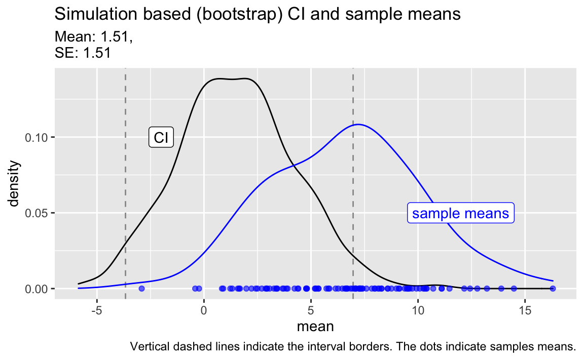
Myth is wrong
Clearly, it is not true that the bulk (95%) of the samples (in blue) fell inside our original 95% CI (in black).
This is clearly spelled out by Danial Kaplan in his book Statistical Modelling:
Another tempting statement is, “If I repeated my study with a different random sample, the new result would be within the margin of error of the original result.” But that statement isn’t correct mathematically, unless your point estimate happens to align perfectly with the population parameter – and there’s no reason to think this is the case.
What is actually true
It is true, however, that - given the assumptions of the model are met - that 95% percent of an infinity of sample CIs will cover the real (mean) of the population.
Does this information help?
Well, some critics say that the CI is rather useless. In fact, Danial Kaplan advises us to nothing more than to interpret the confidence interval in this matter (same page as above):
Treat the confidence interval just as an indication of the precision of the measurement. If you do a study that finds a statistic of 17 ± 6 and someone else does a study that gives 23 ± 5, then there is little reason to think that the two studies are inconsistent. On the other hand, if your study gives 17 ± 2 and the other study is 23 ± 1, then something seems to be going on; you have a genuine disagreement on your hands.