Why you should spell out your model explicitly
Often, assumptions of widely used models, such as linear models, appear opaque. Why is heteroscedasticity important? Where is a list of the model assumptions I need to consider?
As it turns out, there are straight forward answers to these (and similar) questions. The solution is to explicitly spell out your model. All “assumptions” can easily read off from these model specifications.
Example for explicit (and complex) model
Say, we would like to model Covid-19 cases () as a function of tests applied in some population. We could specify our model like this:
Here, we model as Poisson () distribution variable, because is a count variable, and Poisson is a maximum entropy variable for counts. However, this is a apriori reasoning; after seeing the data we might want to consider different model despite the danger of overfitting.
Recall that must be positive or null. That’s why we put a “log” before the likelihood (the linear model specification) line. Similarly, we can only take the log of a positive number, so we need to make sure that . Here, the Exponential distribution () is handy, as it makes sure that or ist positive.
It’s helpful to use standardized predictors, , because that allows us to model the intercept as the mean value of , among other things. It would be a fruitful discussion to contemplate the usefulness of the mean for long-tail distributions, see Taleb Incerto, but that’s beyond the scope of this post.
We must take care of the log-normal (), because log-normal are fat-tailed so the mean will be large. Seeing is believing, so let’s consider . Draw some samples from that population:
set.seed(42)
a <- rlnorm(n = 1000, meanlog = 0, sdlog = 10)
options(scipen = 3)
mean(a)
#> [1] 1716379931934

format(mean(a), scientific = T)
#> [1] "1.71638e+12"
For a smaller sd:
set.seed(42)
a <- rlnorm(n = 1000, meanlog = 4, sdlog = 1)
options(scipen = 3)
mean(a)
#> [1] 88.55222

format(mean(a), scientific = T)
#> [1] "8.855222e+01"
Let’s apply the same reasoning for .
Read off modelling assumptions
Some of the “assumptions” implied by the above model are:
- Certain distributions of the variables involved
- Certain function forms map the input variable to the output variable
- The conditional errors (conditional to ) are iid - independent and identically distributed, that is, at each value of the errors are drawn from the same distribution, and they are drawn without correlation (eg., drawn randomly from an infinite population). This fact incorporated heteroscedasticity, as the residuals have the same variance irrespective to .
- Our ignorance according to the “true” value of some variable is incorporated. For example, we are not sure about the true value of , there is uncertainty involved, which is reflected by the fact that is drawn from a probability distribution.
Simulate data
Say,
According to our model:
set.seed(42)
n <- 1000
alpha <- rexp(n = 1000, rate = 1)
beta <- rexp(n = 1000, rate = 0.1)
See:
ggplot(data.frame(alpha)) +
  aes(x = alpha) +
  geom_density()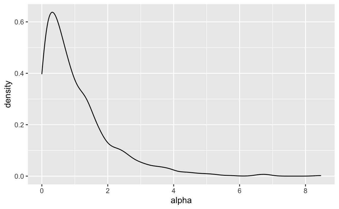
ggplot(data.frame(beta)) +
  aes(x = beta) +
  geom_density()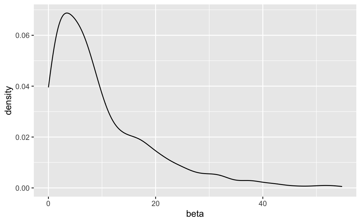
As we do not have real data , we need to simulate it. Assuming that is again exponentially distributed (to avoid negative values):
set.seed(42)
X <- rexp(1000, rate = .5)
ggplot(data.frame(X)) +
aes(x = X) +
geom_density() +
theme_ipsum_rc()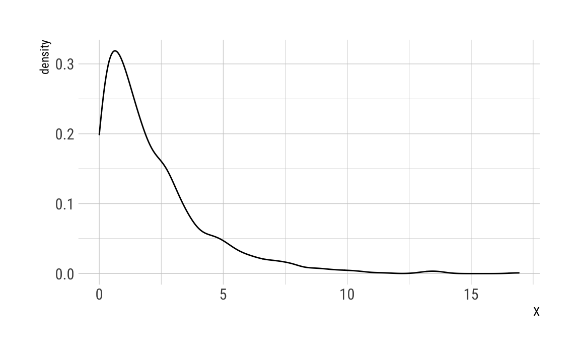
Compute the likelihood
lambda_log <- (alpha + beta*X) %>% log()

lambda <- exp(lambda_log)
ggplot(data.frame(lambda)) +
aes(x = lambda) +
geom_density()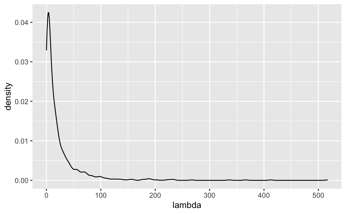
Oh my, that’s a long tail.
Put the data together
C_df <- tibble(
  C = C,
  lambda = lambda,
  lambda_log = lambda_log,
  X = X,
  alpha = alpha,
  beta = beta)
ggplot(C_df) +
aes(x= C) +
geom_density() +
theme_ipsum_rc(grid = "Y")
Fit distributions
pois_param <- fitdistr(C_df$C,
                       densfun = "poisson")$estimate
str(pois_param)
#>  Named num 23.2
#>  - attr(*, "names")= chr "lambda"

pois_param
#> lambda
#> 23.184
Supported distributions are:
“beta”, “cauchy”, “chi-squared”, “exponential”, “gamma”, “geometric”, “log-normal”, “lognormal”, “logistic”, “negative binomial”, “normal”, “Poisson”, “t” and “weibull”
For comparison, let’s fit another distribution, say a log-normal.
lnorm_param <- fitdistr(C_df$C[C_df$C > 0],
                        densfun = "lognormal")$estimate
lnorm_param
#>  meanlog    sdlog
#> 2.389367 1.337632
… or a Gamma:
gamma_param <- fitdistr(C_df$C[C_df$C > 0],
                        densfun = "gamma")$estimate
gamma_param
#>      shape       rate
#> 0.71162128 0.02796269
Compare fit
To compare fit, a qqplot can be helpful.
Poisson
C_df %>%
  ggplot(aes(sample = C)) +
  geom_qq(distribution = qpois,
          dparams = as.list(pois_param),
          color = "dodgerblue") +
  stat_qq_line(distribution = qpois,
               dparams = as.list(pois_param),
               color = "dodgerblue") +
  theme_ipsum_rc()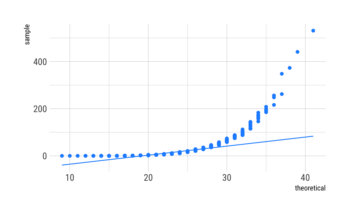
Gamma
C_df %>%
  ggplot(aes(sample = C)) +
  geom_qq(distribution = qgamma,
          dparams = as.list(gamma_param),
          color = "darkseagreen") +
  stat_qq_line(distribution = qgamma,
               dparams = as.list(gamma_param),
               color = "darkseagreen") +
  theme_ipsum_rc()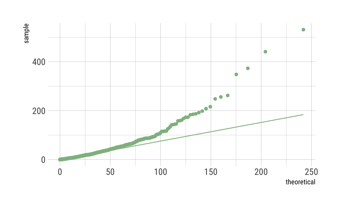
Log-normal
C_df %>%
  ggplot(aes(sample = C)) +
  geom_qq(distribution = qlnorm,
          dparams = as.list(lnorm_param),
          color = "firebrick") +
  stat_qq_line(distribution = qlnorm,
               dparams = as.list(lnorm_param),
               color = "firebrick")  +
  theme_ipsum_rc()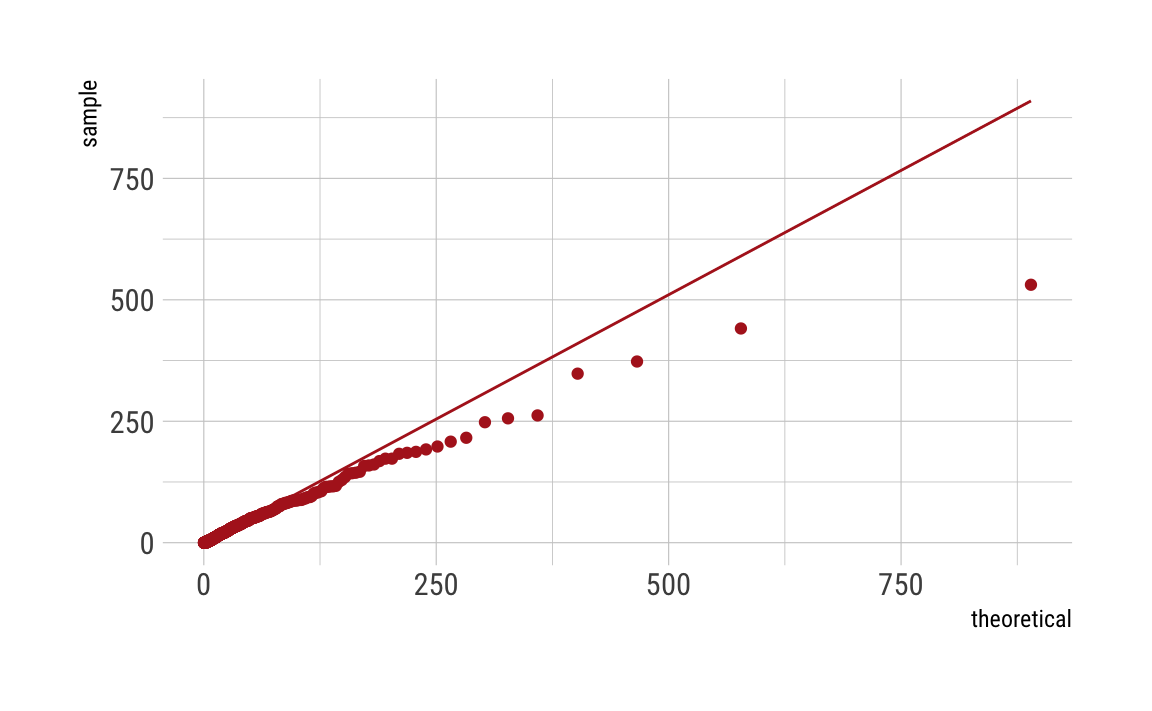
As can be seen, our distributions do not fit well, even given the fact that we simulated the data to be Poisson distributed. This may be due to the fact that we have induced such a long tail. Maybe there are other things going on. Any ideas? Let me know.