Load packages

library(tidyverse)
library(e1071)

My $y$ is not distributed according to my wishes!

Let $Y$ be a variable that we would like to model, for instance, Covid-19 cases.

Now, there’s a widely hold belief that my $Y$ must be distributed normally, or, in some cases, following some other assumed distribution (maybe some long-tailed distribution).

However, this belief is not (strictly) true. What a linear model assumes is that the residuals are distributed normally, not the $Y$ distribution. While this is often left implicit, it is helpful to spell out a model explicitly.

Here’s a simple example from Gelmann and Hill, 2007, p. 46.

Consider a regression with the predictor $X$ , which takes on the values 0, 1, and 2, equally distributed:

$X \sim U_{D} (a = 1, b = 3)$

where $U_{D}$ referes to a discrete uniform distribution with minimum $a$ and maximum $b$ .

Now, let the true association of $X$ and $Y$ amount to:

$y_{i} = 0.2 + 0.5 x_{i}$

Having specified this, we have completely specified this data generating process.

For modelling purposes, let’s add some noise:

$\hat{y_{i}} = 0.2 + 0.5 x_{i} + e_{i} e_{i} \sim N (0, 0.1)$

Simulate some data

Let’s draw a sample of $n = 1000$ .

n <- 1000

set.seed(42)
X <- sample(x = c(1,2,3), size = n, replace = T)
e <- rnorm(n, mean = 0, sd = 0.1)

Compute $Y$ and $\hat{Y}$ :

Y <- 0.2 + 0.5*X

Y_hat <- 0.02 + 0.5*X + e

And put it all in a data frame:

X <- tibble(
  X = X,
  Y = Y,
  Y_hat = Y_hat,
  e = e,
)

Plot the data

X %>%
  ggplot(aes(x = X)) +
  geom_histogram() +
  scale_x_continuous(limits = c(0,3))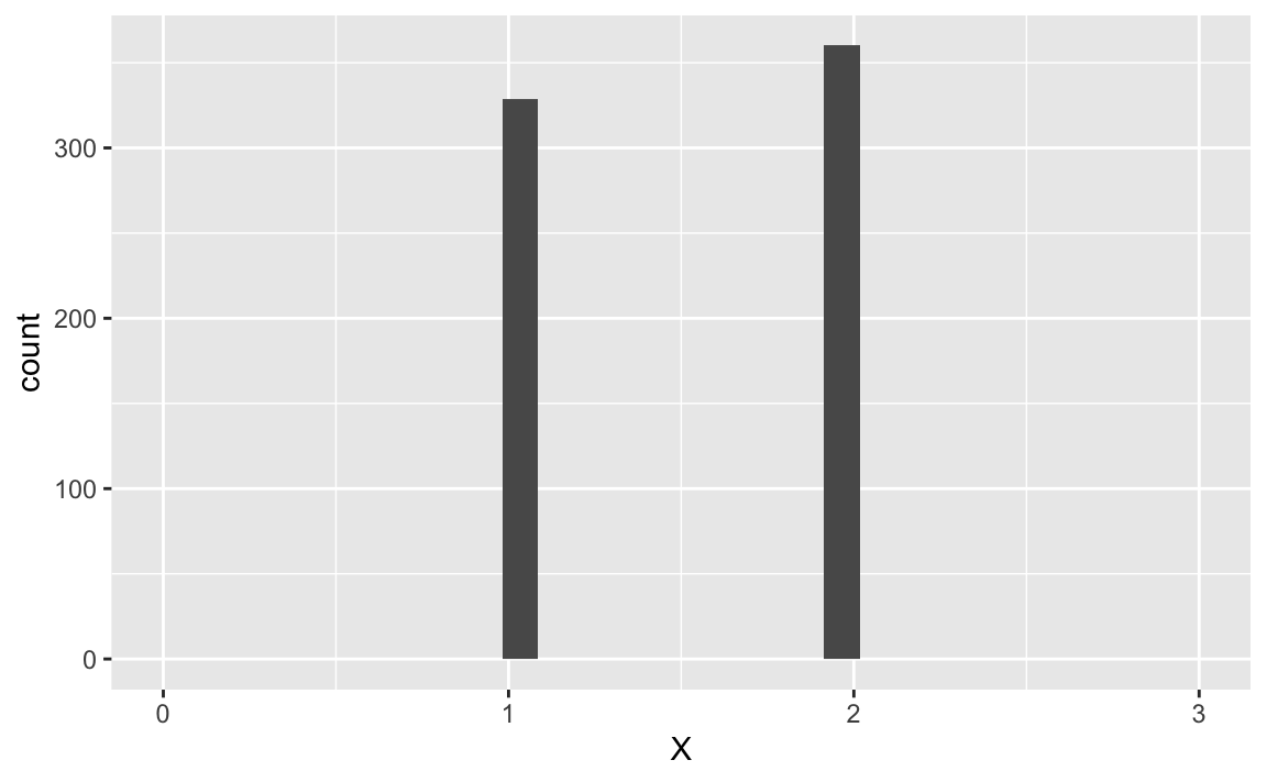

X %>%
  ggplot(aes(x = Y)) +
  geom_histogram() +
  scale_x_continuous(limits = c(0,3))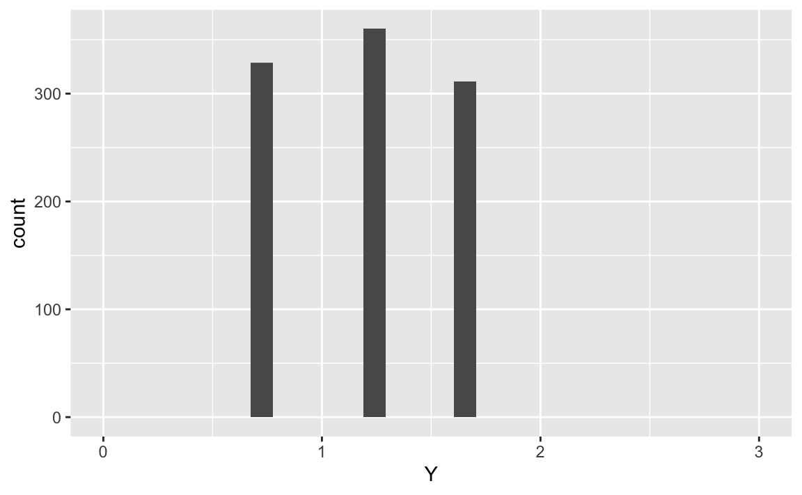

X %>%
  ggplot(aes(x = Y_hat)) +
  geom_histogram() +
  scale_x_continuous(limits = c(0,3))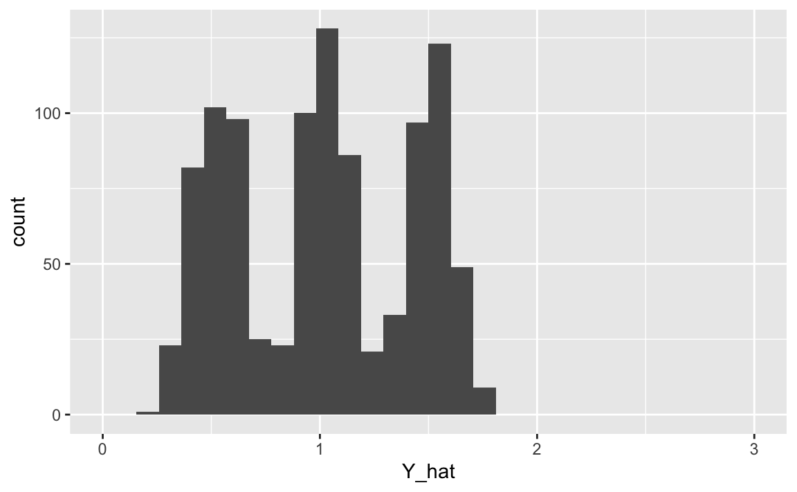

X %>%
  ggplot(aes(x = e)) +
  geom_histogram() +
  scale_x_continuous(limits = c(-3,3))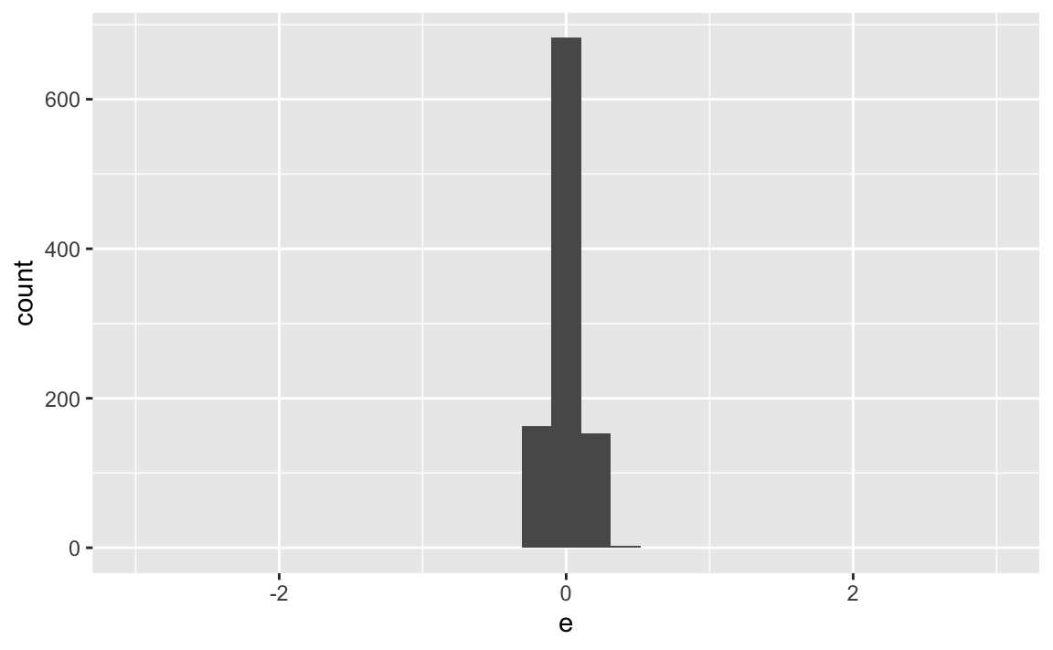

And interstingly, $e_{i} | X_{i}$ :

X %>%
  ggplot(aes(x = e, group = X, 
             color = factor(X))) +
  geom_density()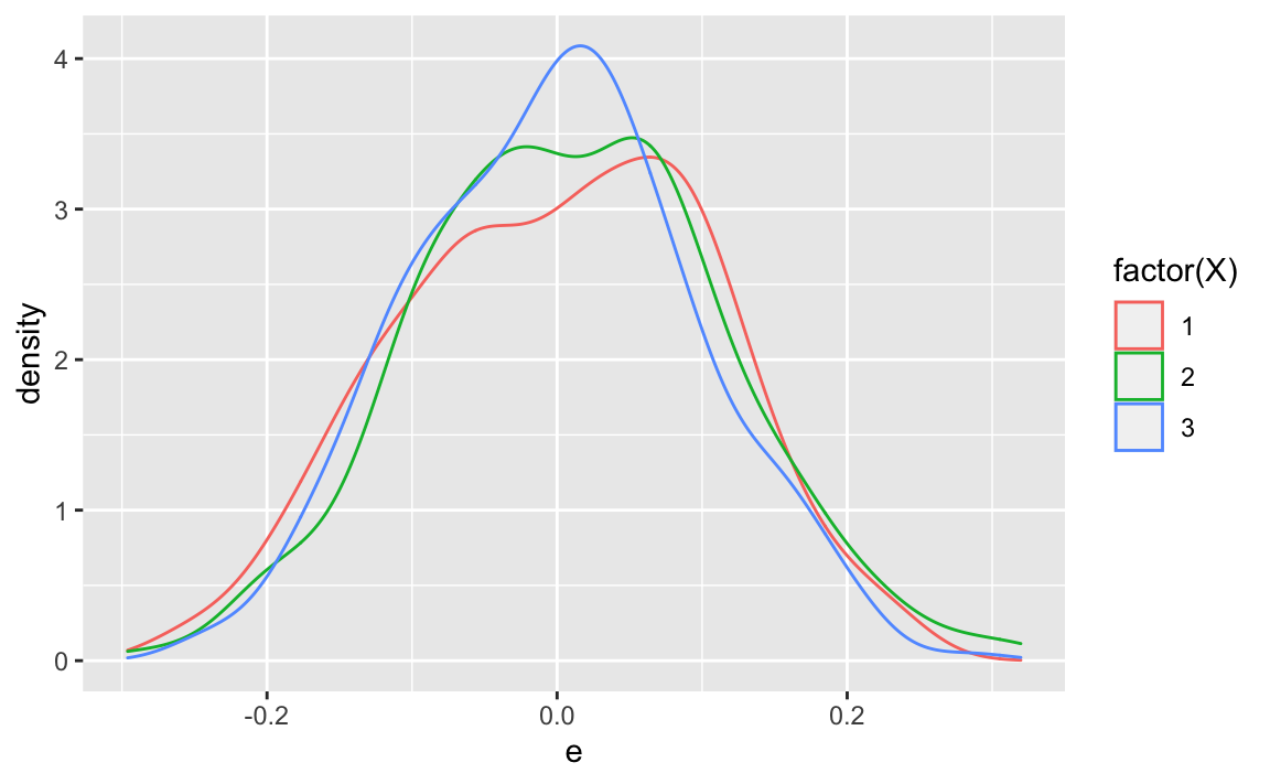

Compare that to $e$ , the unconditional (marginal) error distribution:

X %>%
  ggplot(aes(x = e)) +
  geom_density()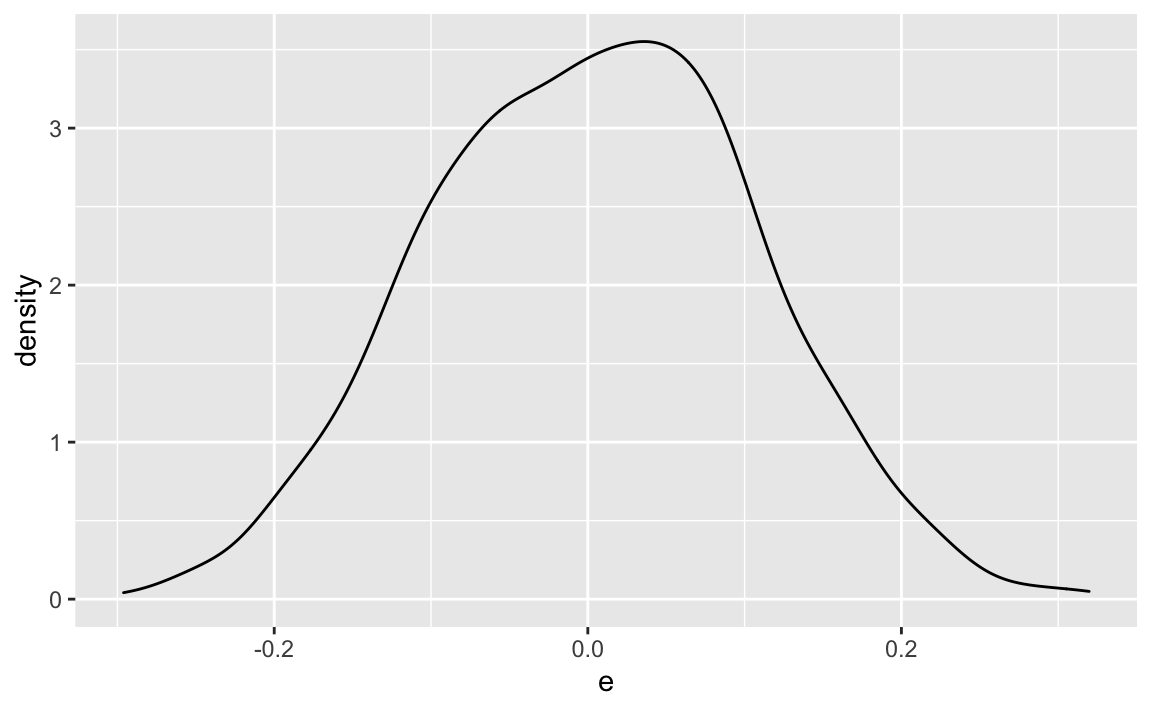

Quite similar, but: do we have thicker tails in $e$ compared to $e | X$ ? We have effectively mixed three distributions,so we might expect fatter tails.

e1071::kurtosis(X$X)
#> [1] -1.439171

Recall that the kurtosis of the normal distribution is 3.

As a side note (same source as above):

It is also common practice to use an adjusted version of Pearson’s kurtosis, the excess kurtosis, which is the kurtosis minus 3, to provide the comparison to the normal distribution.

Some authors use “kurtosis” by itself to refer to the excess kurtosis. For clarity and generality, however, this article follows the non-excess convention and explicitly indicates where excess kurtosis is meant.

The function kurtosis provides the standard form of kurtosis, where normal distributed variables have a value of 3.

Compare that to the conditional kurtosis $Y | X$ :

X %>% 
  group_by(X) %>% 
  summarise(kurtY = kurtosis(e))
#> # A tibble: 3 x 2
#>       X   kurtY
#>   <dbl>   <dbl>
#> 1     1 -0.615 
#> 2     2 -0.0636
#> 3     3 -0.319

There does not appear to be any difference in the kurtosis between $e$ and $e | X$ .

Conclusion 1

The distribution of $Y$ is not of importance when it comes to the assumptions a linear models. However, the distribution of residuals (“errors”) is of some importance.

Conclusion 2: Fuhgetaboutit, says Gelman

However, Gelman (same source as above) tells us that

assumption of normality is barely important at all.

(p. 46)

As a consequence

we do not recommend diagnostics of the normality of regression residuals.

(italics in original)

Debrief

The distribution of $Y$ does not need to be similar to the distribution of the modelling residuals. There’s no need to check the $Y$ distribution, at least not for modelling purposes (for regression type models).

Distribution of residuals is of interest for linear models, not the distribution of y