Load packages
library(tidyverse)
library(mosaic)
Data
data("tips", package = "reshape2")Non-parametric tests and simulation based inference
Simulation-based inference (SBI) is an old tool that has seen a surge in research interest in recent years probably due to the large amount of computational powers at the hands of researchers.
SBI is less prone to violations of assumptions, particularly with distributional assumptions. This is because inference is not based on the idea that some variable follows a – for example – normal distribution.
As a consequence there is much less need to seek shelter at nonparametric tests in case distributional assumptions are violated.
In this post, I’ll show how the Kurskal-Wallis test can be applied using SBI and how to translate it to a linear model.
Research question
Is there a difference in mean tip across different days?
Kruskall test the classic way
k_test <- kruskal.test(tip ~ day, data = tips)
k_test
#>
#>  Kruskal-Wallis rank sum test
#>
#> data:  tip by day
#> Kruskal-Wallis chi-squared = 8.5656, df = 3, p-value = 0.03566
Let’s have a closer look to the resulting object:
str(k_test)
#> List of 5
#>  $ statistic: Named num 8.57
#>   ..- attr(*, "names")= chr "Kruskal-Wallis chi-squared"
#>  $ parameter: Named int 3
#>   ..- attr(*, "names")= chr "df"
#>  $ p.value  : num 0.0357
#>  $ method   : chr "Kruskal-Wallis rank sum test"
#>  $ data.name: chr "tip by day"
#>  - attr(*, "class")= chr "htest"
We can extract the statistic in this way:
k_test$statistic
#> Kruskal-Wallis chi-squared
#>                   8.565588
pluck(k_test, "statistic")
#> Kruskal-Wallis chi-squared
#>                   8.565588
Or, alternatively:
kruskal.test(tip ~ day, data = tips)$statistic
#> Kruskal-Wallis chi-squared
#>                   8.565588
The statistic is defined as shown here:
\[ H = (N-1)\frac{\sum_{i=1}^g n_i(\bar{r}_{i\cdot} - \bar{r})^2}{\sum_{i=1}^g\sum_{j=1}^{n_i}(r_{ij} - \bar{r})^2} \]
And this statistic is asymptotically \(\chi^2\) distributed.
Kruskall test via SBI
null1 <- mosaic::do(1000) * kruskal.test(tip ~ shuffle(day),
                                 data = tips)
Let’s check the results:
null1 %>%
  head() %>%
knitr::kable()| Kruskal.Wallis.chi.squared | df | p.value | method | alternative | data | .row | .index |
|---|---|---|---|---|---|---|---|
| 3.1688452 | 3 | 0.3663180 | Kruskal-Wallis rank sum test | NA | tip by shuffle(day) | 1 | 1 |
| 0.0094803 | 3 | 0.9997552 | Kruskal-Wallis rank sum test | NA | tip by shuffle(day) | 1 | 2 |
| 11.7318235 | 3 | 0.0083606 | Kruskal-Wallis rank sum test | NA | tip by shuffle(day) | 1 | 3 |
| 4.3075100 | 3 | 0.2301161 | Kruskal-Wallis rank sum test | NA | tip by shuffle(day) | 1 | 4 |
| 1.5435937 | 3 | 0.6722461 | Kruskal-Wallis rank sum test | NA | tip by shuffle(day) | 1 | 5 |
| 1.4203264 | 3 | 0.7007771 | Kruskal-Wallis rank sum test | NA | tip by shuffle(day) | 1 | 6 |
Plot it
Let’s add the empirical value as a vertical line.
gf_histogram( ~ Kruskal.Wallis.chi.squared, data = null1) %>%
  gf_vline(xintercept = ~ k_test$statistic)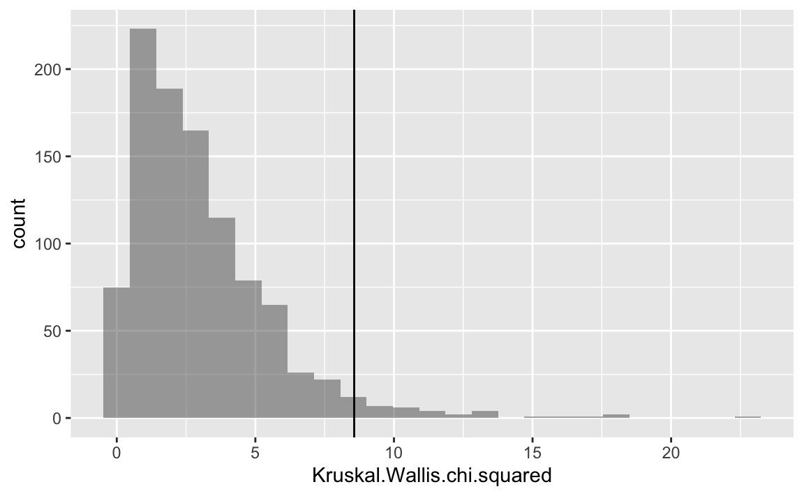
Let’s color the top-5 percent red, to highlight the critical value.
null1 <- null1 %>%
  mutate(is_top5percent = percent_rank(Kruskal.Wallis.chi.squared)  > .95)
gf_histogram( ~ Kruskal.Wallis.chi.squared,
data = null1,
fill = ~ is_top5percent) %>%
gf_vline(xintercept = ~ k_test$statistic)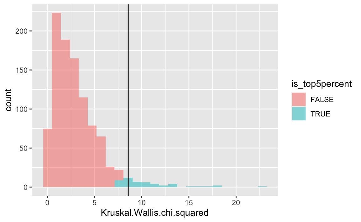
Nice, but …
As outlined above, there may be no need to bypass the test of the mean. Using SBI one does not have to assume normal distribution of the variable tested if one would like to compute p-values.
Linear model for comparing means
lm1 <- lm(tip ~ day, data = tips)
lm1_sum <- summary(lm1)

lm1_sum
#>
#> Call:
#> lm(formula = tip ~ day, data = tips)
#>
#> Residuals:
#>     Min      1Q  Median      3Q     Max
#> -2.2451 -0.9931 -0.2347  0.5382  7.0069
#>
#> Coefficients:
#>             Estimate Std. Error t value Pr(>|t|)
#> (Intercept)  2.73474    0.31612   8.651 7.46e-16 ***
#> daySat       0.25837    0.34893   0.740    0.460
#> daySun       0.52039    0.35343   1.472    0.142
#> dayThur      0.03671    0.36132   0.102    0.919
#> ---
#> Signif. codes:  0 '***' 0.001 '**' 0.01 '*' 0.05 '.' 0.1 ' ' 1
#>
#> Residual standard error: 1.378 on 240 degrees of freedom
#> Multiple R-squared:  0.02048,    Adjusted R-squared:  0.008232
#> F-statistic: 1.672 on 3 and 240 DF,  p-value: 0.1736
As can be seen, the \(F\) value is not significant thereby questioning the difference in means hypothesis. Put differently: The models sees no strong evidence for rejecting the null.
The F value, along with its 3 df values, can be plucked out like this:
emp_F_value <- pluck(lm1_sum, "fstatistic")
emp_F_value
#>      value      numdf      dendf
#>   1.672355   3.000000 240.000000
Note that this is a vector of three 3 elements.
Linear model using SBI
Now the trick.
boot1 <- do(1000) * lm(tip ~ day, data = resample(tips))

confint(boot1)
#>        name        lower     upper level     method   estimate
#> 1 Intercept  2.270318182 3.2140346  0.95 percentile 2.73473684
#> 2    daySat -0.304165972 0.8272075  0.95 percentile 0.25836661
#> 3    daySun  0.030470180 1.0744534  0.95 percentile 0.52039474
#> 4   dayThur -0.480811080 0.6252964  0.95 percentile 0.03671477
#> 5     sigma  1.157816369 1.5729610  0.95 percentile 1.37793112
#> 6 r.squared  0.005899732 0.0758314  0.95 percentile 0.02047639
#> 7         F  0.474779633 6.5642919  0.95 percentile 1.67235520
Pluck the r-squared from the lm object
Here’s a way to pluck the R squared value from the lm object:
lm(tip ~ day, data = tips) %>%
  summary() %>%
  pluck("r.squared")
#> [1] 0.02047639
Plot the results
gf_histogram(~ r.squared, data = boot1) %>%
  gf_vline( xintercept = ~ lm(tip ~ day, data = tips) %>%
              summary() %>%
              pluck("r.squared"))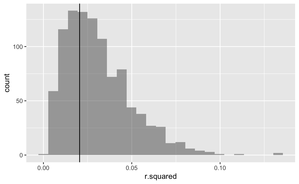
Interestingly, the R squeared distribution is not normally distributed. In sum, the R squared are really small.
Test the null using lm and SBI
null2 <- do(1000) * lm(tip ~ shuffle(day), data = tips)Let’s check the \(F\) statistic. The critical value of the \(F\) statistic is, given 3 and 240 degrees of freedom (as shown by the lm output):
crit_f <- qf(p = 0.95,
             df1 = 3,
             df2 = 240)
crit_f
#> [1] 2.642213
Plot it:
null2 <- null2 %>%
  mutate(top_5percent = percent_rank(F) > 0.95)

gf_histogram(~ F, data = null2,
             fill =~top_5percent) %>%
  gf_vline(xintercept = ~emp_F_value[1]) %>%
  gf_label(label = ~ paste0("F: ",
                            emp_F_value[1] %>% round(2)),
           x = ~ emp_F_value[1],
           y = 0,
show.legend = FALSE) 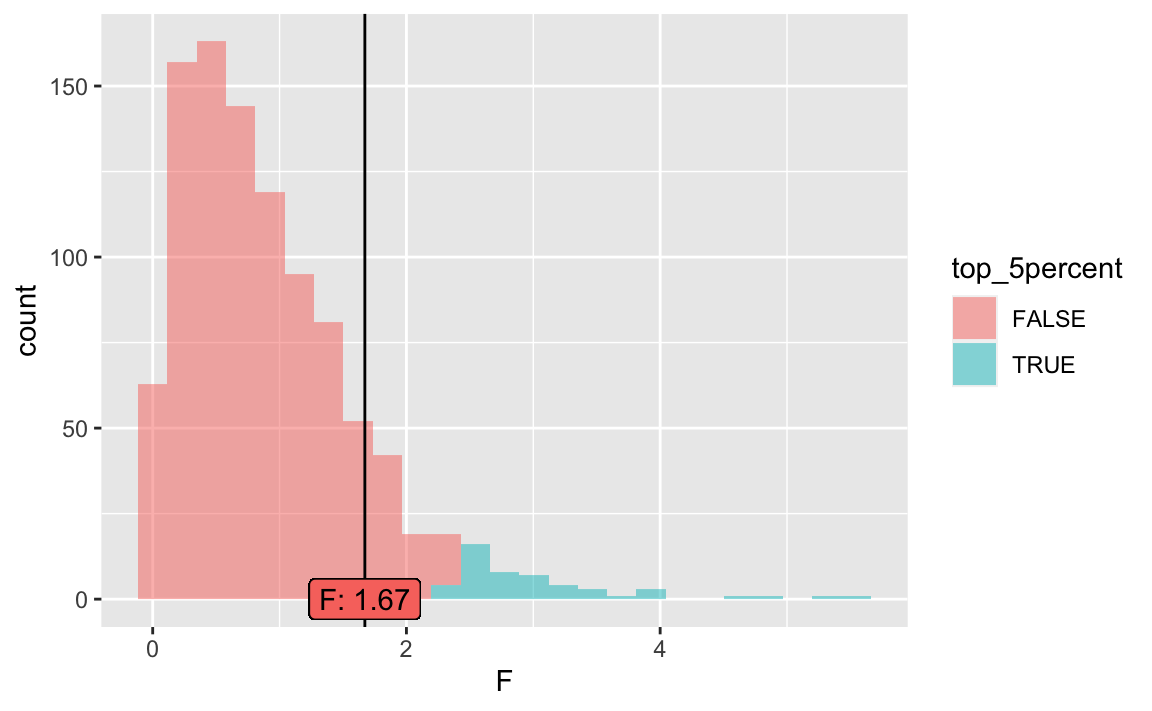
As can be seen, the F value is not significant.
Some summary statistics to this distribution:
favstats(~ F, data = null2)
#>          min        Q1    median       Q3      max      mean        sd    n
#>  0.006571185 0.3887514 0.7581193 1.293386 5.553417 0.9314424 0.7433274 1000
#>  missing
#>        0
Caution
Note that the ASA advises that the p-value should not be the (sole) basis of decision in any data analysis.
Bayesian statistics is a neat alternative.
ANOVA
As can be seen, the Kruskal Wallis and the F tests yield different results. This is probably due to the fact that we tested median differences (Kruskall) and later on mean differences (F test).
As a check, here’s a standard ANOVA:
aov1 <- aov(tip ~ day, data = tips)
summary(aov1)
#>              Df Sum Sq Mean Sq F value Pr(>F)
#> day           3    9.5   3.175   1.672  0.174
#> Residuals   240  455.7   1.899
Replicating the F value decision from the SBI analysis above.
Plotting medians vs means
As a further check, let’s plot median and mean differences for the sake of comparison.
gf_point(tip ~ day,
         data = tips,
         stat = "summary",
         fun = mean,
         shape = 3,
         size = 5,
         color = "blue") +
  stat_summary(geom = "point",
               fun = median,
               color = "red",
               size = 5,
               shape = 5) +
  labs(caption = "Crosses: Mean, diamonds: Median")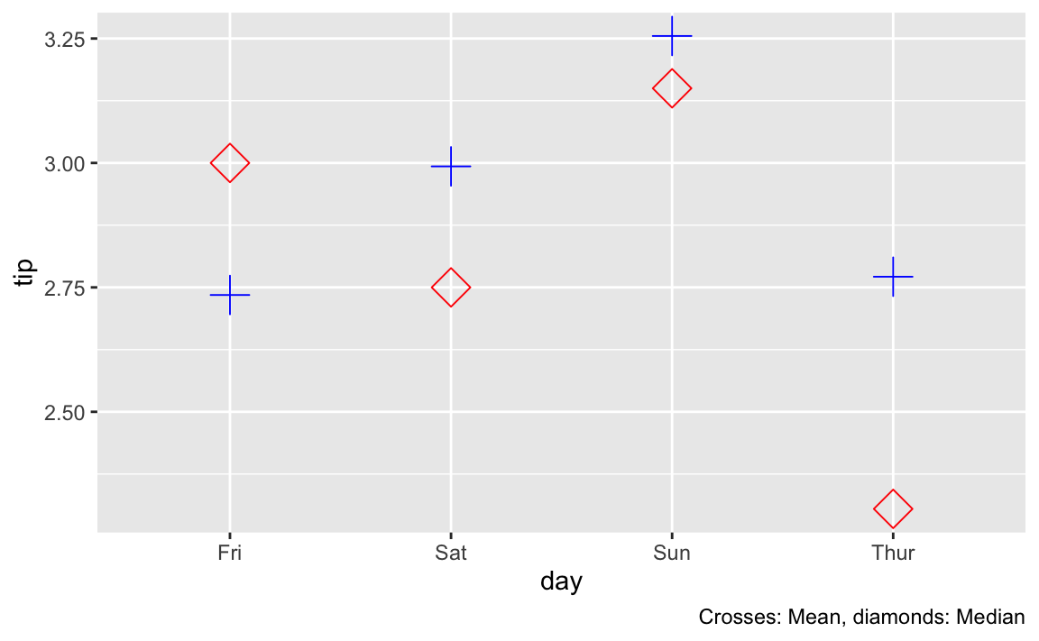
As ca be seen, the median values are more spread out, hence it appears sensible that the test would get significant whereas the more clustered mean values do not show a significant difference in our test.