Load packages

library(tidyverse)
library(conflicted)
library(ggdag)
library(broom)
library(GGally)

Motivation

Assume there is some scientist with some theory. Her theory holds that X and Z are causes of Y. dag1 shows her DAG (ie., her theory depicted as a causal diagram). Our scientist is concerned with the causal effect of X on Y, where X is a treatment variable (exposure) and Y is the dependent variable under scrutiny (outcome).

See e.g,. here or here for intros to DAGs and causality.

DAGs

Let’s define this DAG, first as a plain string (text):

dag1_txt <- "dag {
X -> Y
Z -> Y
X [exposure]
Y [outcome]
}"

Define a DAG representation:

dag1 <- dagitty::dagitty(dag1_txt)
dag1
#> dag {
#> X [exposure]
#> Y [outcome]
#> Z
#> X -> Y
#> Z -> Y
#> }

Make it tidy:

dag1_tidy <- tidy_dagitty(dag1)
dag1_tidy
#> # A DAG with 3 nodes and 2 edges
#> #
#> # Exposure: X
#> # Outcome: Y
#> #
#> # A tibble: 3 x 8
#>   name      x     y direction to     xend  yend circular
#>   <chr> <dbl> <dbl> <fct>     <chr> <dbl> <dbl> <lgl>   
#> 1 X      33.4  30.2 ->        Y      34.3  29.5 FALSE   
#> 2 Z      35.3  28.9 ->        Y      34.3  29.5 FALSE   
#> 3 Y      34.3  29.5 <NA>      <NA>   NA    NA   FALSE

And plot it:

ggdag(dag1_tidy) + theme_dag()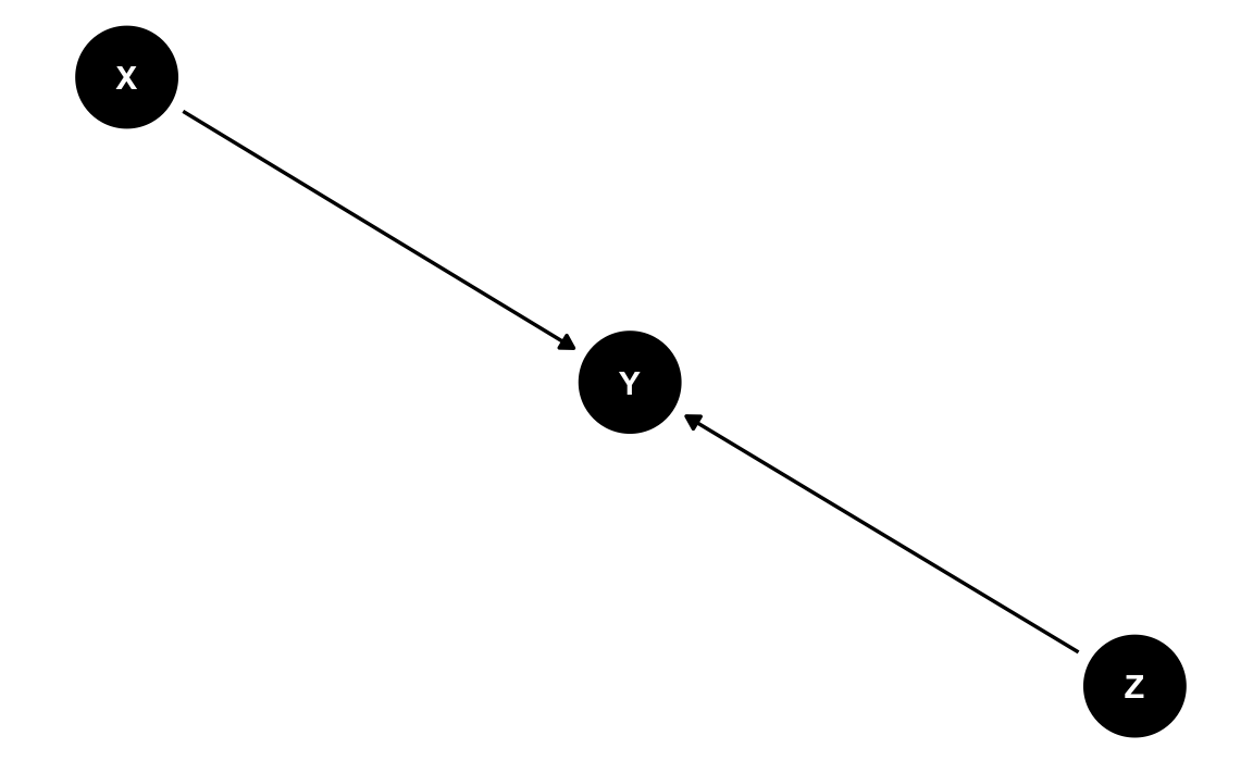

So far, so good. Now, sadly, unbeknownst to our scientist, her theory is actually wrong. Wrong as in wrong. The true theory – only known by Paul Meehl – is depicted by the following dag:

dag2_txt <- "dag {
X -> Z
Y -> Z
X [exposure]
Y [outcome]
}"

dag2_txt
#> [1] "dag {\nX -> Z\nY -> Z\nX [exposure]\nY [outcome]\n}"

dag2_tidy <- dag2_txt %>% dagitty::dagitty() %>% tidy_dagitty()

ggdag(dag2_tidy) + theme_dag()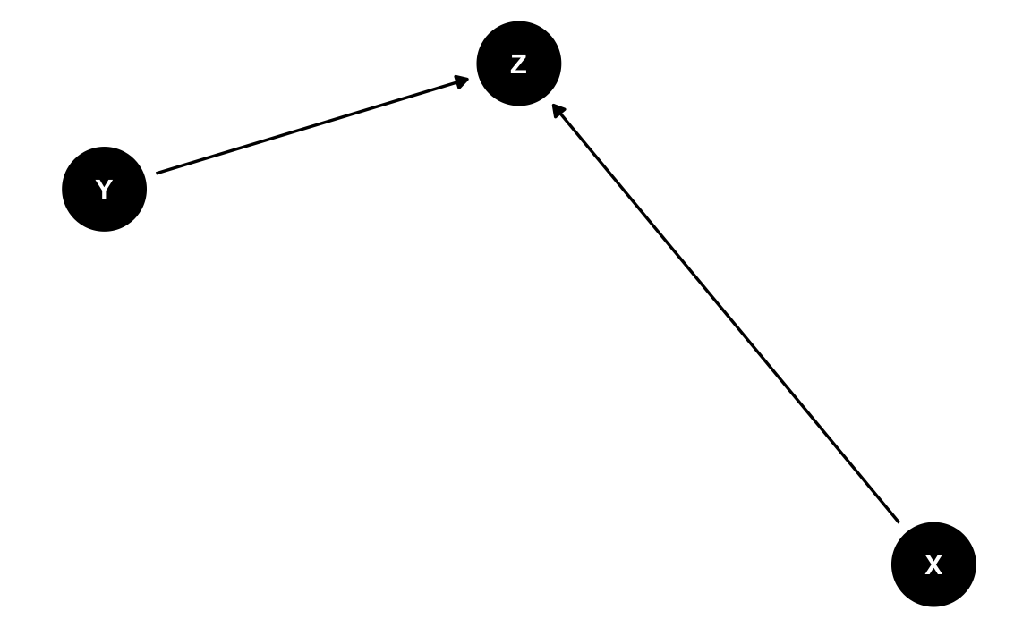

Simulate some data

To make it more concrete, let’s come up with some simulated data according to the true model as depicted in DAG2.

Let’s define this structural causal model as follows.

\[ X \sim Norm(0, 1)\\ Y \sim Norm(0, 1)\\ e \sim Norm(0,0.5)\\ Z = 0.5 X + 0.5Y + e \]

Here Norm means the Normal distribution.

Now let’s draw say \(n=1000\) observations from these distributions:

n <- 1000
X <- rnorm(n, mean = 0, sd = 1)
Y <- rnorm(n, mean = 0, sd = 1)
e <- rnorm(n, mean = 0, sd = 0.5)
Z = 0.5*X + 0.5*Y + e

d <- tibble(X = X, 
            Y = Y, 
            e = e, 
            Z = Z)
glimpse(d)
#> Rows: 1,000
#> Columns: 4
#> $ X <dbl> 0.04256036, -2.51827371, 0.70285885, -0.12464830, -1.61776654, -0.2…
#> $ Y <dbl> -0.07430878, -0.85320737, 0.03305014, 2.66740399, 0.32557657, 0.793…
#> $ e <dbl> 0.661375970, -0.519174385, 0.428588030, 0.186427092, -1.036197797, …
#> $ Z <dbl> 0.64550176, -2.20491492, 0.79654252, 1.45780494, -1.68229278, 0.198…

Regression time

Our scientist has proudly finished her data collection. Now, analysis time, here favorite passe temps.

First, she checks the zero-order (marginal) correlations, ’cause we can:

cor(d)
#>             X            Y            e         Z
#> X  1.00000000 -0.062874185  0.033431583 0.5639263
#> Y -0.06287419  1.000000000 -0.009696558 0.5485886
#> e  0.03343158 -0.009696558  1.000000000 0.5967447
#> Z  0.56392634  0.548588574  0.596744684 1.0000000

ggpairs(d)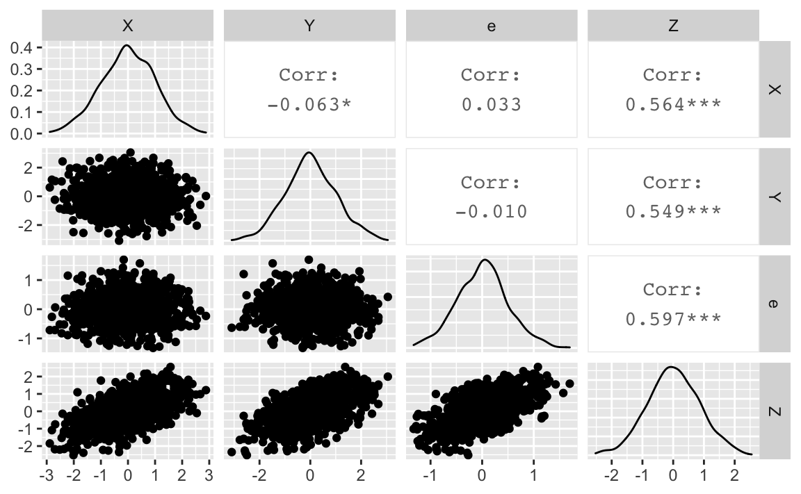

Oh no - bad news. X and Y are not correlated. But, being a well trained data analyst, our scientist keeps the spirits up. She knows that a different way of analysis may well turn a previous result inside out (although sometimes you better not tell what you did in the first place, her supervisor kept on saying, behind closed doors at least).

Here’s the regression of Y back on X:

lm0 <- lm(Y ~ X, data = d)

tidy(lm0)
#> # A tibble: 2 x 5
#>   term        estimate std.error statistic p.value
#>   <chr>          <dbl>     <dbl>     <dbl>   <dbl>
#> 1 (Intercept)   0.0189    0.0317     0.594  0.553 
#> 2 X            -0.0639    0.0321    -1.99   0.0468

Same story as with the marginal correlation above: No association of X and Y.

Now stay tuned: lm1

Here’s the regression according to her model:

lm1 <- lm(Y ~ X + Z, data = d)

tidy(lm1)
#> # A tibble: 3 x 5
#>   term         estimate std.error statistic   p.value
#>   <chr>           <dbl>     <dbl>     <dbl>     <dbl>
#> 1 (Intercept)  0.000193    0.0224   0.00862 9.93e-  1
#> 2 X           -0.554       0.0274 -20.2     2.12e- 76
#> 3 Z            1.01        0.0319  31.7     3.58e-153

Yeah! There is a significant effect of X on Y! Success! Smelling tenure. Now she’ll write up the paper stating that there is “presumably” and “well supported by the data” an “effect” of X on Y. (She doesn’t explicitly calls it a “causal” effect, but hey, what’s an effect if not causal? Ask the next person you happen to run into on the street.)

Stop for a while

The story could be finished here. Alas, in most real cases the story is finished here: manuscript drafted, paper published, sometines tenured.

However, as we know - because we defined it above - her model is wrong. So let’s pause for a while to reflect what happened.

Correct regression

Here’s a (more) correct regression model:

lm2 <- lm(Z ~ X + Y, data = d)

tidy(lm2)
#> # A tibble: 3 x 5
#>   term        estimate std.error statistic   p.value
#>   <chr>          <dbl>     <dbl>     <dbl>     <dbl>
#> 1 (Intercept)  0.00909    0.0157     0.579 5.63e-  1
#> 2 X            0.517      0.0159    32.5   1.58e-158
#> 3 Y            0.496      0.0156    31.7   3.58e-153

The coefficients in our sample turn out nicely just like we had defined the parameters before hand. As we know that DAG2 is true we can have confidence in this present regression model, lm2.

That’s also a valid model:

lm3 <- lm(Z ~ X, data = d)

tidy(lm3)
#> # A tibble: 2 x 5
#>   term        estimate std.error statistic  p.value
#>   <chr>          <dbl>     <dbl>     <dbl>    <dbl>
#> 1 (Intercept)   0.0184    0.0222     0.830 4.07e- 1
#> 2 X             0.485     0.0225    21.6   5.06e-85

As can be seen, the coefficient of X did not change (substantially) in comparison to lm2.

Similarly:

lm4 <- lm(Z ~ Y, data = d)

tidy(lm4)
#> # A tibble: 2 x 5
#>   term        estimate std.error statistic  p.value
#>   <chr>          <dbl>     <dbl>     <dbl>    <dbl>
#> 1 (Intercept)  0.00784    0.0225     0.349 7.27e- 1
#> 2 Y            0.464      0.0224    20.7   1.18e-79

Take home message 3

Sometimes adding a predictor to a regression model hurts. Learn to let go.

What about this regression model?

lm5 <- lm(Y ~ X, data = d)

tidy(lm5)
#> # A tibble: 2 x 5
#>   term        estimate std.error statistic p.value
#>   <chr>          <dbl>     <dbl>     <dbl>   <dbl>
#> 1 (Intercept)   0.0189    0.0317     0.594  0.553 
#> 2 X            -0.0639    0.0321    -1.99   0.0468

This model is O.K. too. Check the DAG: The DAG tells us that there’s no causal effect from X onto Y. The regression model supports that notion.

Debrief

The story above only holds if one tries to estimate a causal effect. It’s a completely different story if someone “only” would like to predict some variable, say Y.

Prediction has its value, of course. Call me if you are able to predict tomorrows DAX value.

For science however, prediction is of little value in many times. Rather, we would like to understand why a correlation takes place. What do we learn by knowing that babies and storks are correlated? Nothing. Why not? And why is it easy to accept? Because we intuitively know that there’s no causation going on here. That’s the crucial point. Absent causal information, we do not learn much or maybe nothing from a correlation.

A last example

Say you learn that chocolate consumption and (number of) Nobel laureates (per country) is correlated (see this source by Fabian Dablander). Interesting?! Of course, that’s again an example of “too strange to be true”. As a rule of thumb, if it’s too strange to be true it’s probably not true. One explanation could be that in “developed” countries (whatever that is) there’s a high chocolate consumption and a (relatively) high number of Nobel laureates. In not-so-developed countries the reverse is true. Hence, there’s a correlation of development status and chocolate consumption. And a correlation of development status and Nobel laureates. In fact, not only correlation but causation by virtue of this example. Now, as we are aware of the true “background” – the development status – as the driver of the “unreal” (spurious) correlation between chocolate and Nobel stuff, we know that this spurious correlation is of ZERO value (for understanding what’s going on). How do we know? Because we now know that there’s no causal association between chocolate and Nobel stuff. But there is a causal association between development status and the other two variables.