Load packages

library(tidyverse)

Motivation

This post is a compilation, rather uncommented compilation, of various methods of plotting 3D (bivariate) Gaussian distributions in R.

I add the source to each method.

Note that some methods (5, 6) open a interactive window wihich is not supported here. I added a static version of the plot then.

Method 1

Source: https://codegolf.stackexchange.com/questions/123039/plot-the-gaussian-distribution-in-3d

Feel free to change the sd, s in the code below.

s=1

plot3D::persp3D(z=sapply(x<-seq(-6,6,.1),
                         function(y)exp(-(y^2+x^2)/(2*s^2))))

Method 2

Same source as above.

Using plotly, as more stylish:

s = 2
plotly::plot_ly(z=sapply(x<-seq(-6,6,.1),
                         function(y)exp(-(y^2+x^2)/(2*s^2))),x=x,y=x,type="surface")

Method 3

Source: https://stat.ethz.ch/pipermail/r-help/2006-January/087045.html

x <- y <- seq(-5, 5, len = 200)
X <- expand.grid(x = x, y = y)
X <- transform(X, z = dnorm(x, -2.5)*dnorm(y) - dnorm(x, 2.5)*dnorm(y))
z <- matrix(X$z, nrow = 200)

persp(x, y, z, col = "lightgoldenrod", border = NA,
      theta = 30, phi = 15, ticktype = "detailed", 
      ltheta = -120, shade = 0.25)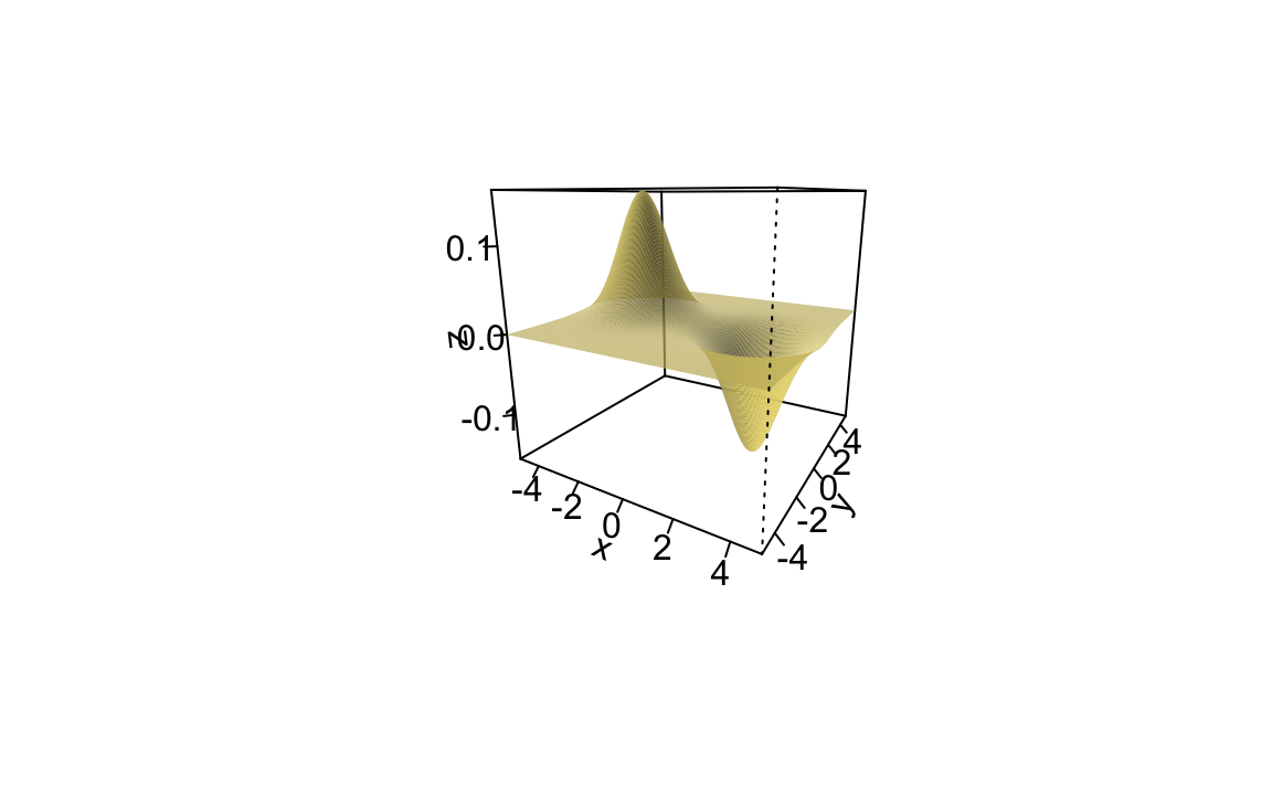

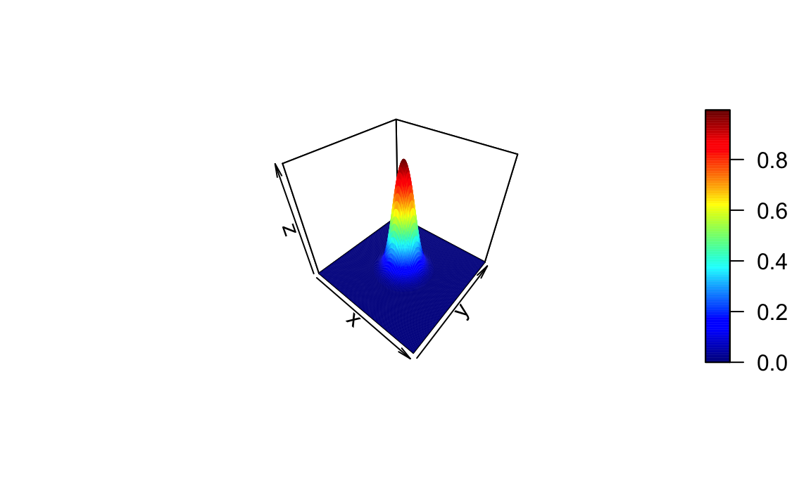
Method 4

Source: https://stackoverflow.com/questions/36125313/3d-plot-of-normal-distribution-in-r-around-a-x-y-point

library(rgl)
open3d()
#> glX 
#>   1

x <- seq(0, 10, length=100)
y <- seq(0, 10, length=100)


z = outer(x,y, function(x,y) dnorm(x,5,1)*dnorm(y,5,1))

persp3d(x, y, z,col = rainbow(100))

Method 5

Same source as above.

library(rgl)
open3d()
#> glX 
#>   2
z = outer(x,y, function(x,y) dnorm(x,2.5,1))
persp3d(x, y, z,col = rainbow(100))


volcano<-function(x,y,sigma=1/2) {
  alpha<-atan(y/x)+pi*(x<0)
  d<-sqrt((cos(alpha)-x)^2 + (sin(alpha)-y)^2)
  dnorm(d,0,sigma)
}
x<-seq(-2,2,length.out=100)
y<-seq(-2,2,length.out=100)
z<-outer(x,y,volcano)
persp3d(x, y, z,col = rainbow(100))

Method 6

Source: http://www.countbio.com/web_pages/left_object/R_for_biology/R_fundamentals/3D_surface_plot_R.html

##  2D Gaussian Kernal plot

## Generate x and y coordinates as sequences
x = seq(-4,4,0.2)
y = seq(-4,4,0.2)

# An empty matrix z
z = matrix(data=NA, nrow=length(x), ncol=length(x))

### Gaussian kernal generation to fill the z matrix.
sigma = 1.0
mux = 0.0
muy = 0.0
A = 1.0

for(i in 1:length(x))
{
  for(j in 1:length(y))
  {
    
    z[i,j] = A * (1/(2*pi*sigma^2)) * exp( -((x[i]-mux)^2 + (y[j]-muy)^2)/(2*sigma^2)) 
  }
}


library(plot3D)
persp3D(x,y,z,theta=30, phi=50, axes=TRUE,scale=2, box=TRUE, nticks=5, 
        ticktype="detailed", xlab="X-value", ylab="Y-value", zlab="Z-value", 
        main="Gaussian Kernal with persp3D()")

Method 7

Same source as above.

library(threejs)
library(MASS)

mu <- c(0,0)                         # Mean
Sigma <- matrix(c(1, .5, .5, 1), 2)  # Covariance matrix
# > Sigma
# [,1] [,2]
# [1,]  1.0  0.1
# [2,]  0.1  1.0

bivn <- mvrnorm(5000, mu = mu, Sigma = Sigma )  # from Mass package
head(bivn)                                      
#>            [,1]         [,2]
#> [1,] -0.3874662 -0.249706809
#> [2,]  0.4892134  0.972939902
#> [3,]  0.3566242 -0.092561697
#> [4,]  0.2890245  0.004173115
#> [5,]  1.8616669  1.865217470
#> [6,]  0.1448117  1.750661575
# Calculate kernel density estimate
bivn.kde <- kde2d(bivn[,1], bivn[,2], n = 50)




# Unpack data from kde grid format
x <- bivn.kde$x; y <- bivn.kde$y; z <- bivn.kde$z
# Construct x,y,z coordinates
xx <- rep(x,times=length(y))
yy <- rep(y,each=length(x))
zz <- z; dim(zz) <- NULL
# Set up color range
ra <- ceiling(16 * zz/max(zz))
col <- rainbow(16, 2/3)
# 3D interactive scatter plot
scatterplot3js(x=xx,y=yy,z=zz,size=0.4,color = col[ra],bg="black")

Method 8

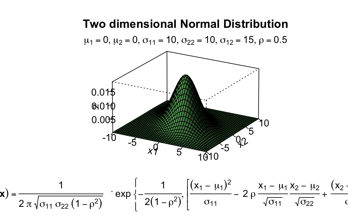
Source: https://www.ejwagenmakers.com/misc/Plotting_3d_in_R.pdf

# 3-D plots
#
#
mu1<-0 # setting the expected value of x1
mu2<-0 # setting the expected value of x2
s11<-10 # setting the variance of x1
s12<-15 # setting the covariance between x1 and x2
s22<-10 # setting the variance of x2
rho<-0.5 # setting the correlation coefficient between x1 and x2
x1<-seq(-10,10,length=41) # generating the vector series x1
x2<-x1 # copying x1 to x2
#
f<-function(x1,x2)
{
  term1<-1/(2*pi*sqrt(s11*s22*(1-rho^2)))
  term2<--1/(2*(1-rho^2))
  term3<-(x1-mu1)^2/s11
  term4<-(x2-mu2)^2/s22
  term5<--2*rho*((x1-mu1)*(x2-mu2))/(sqrt(s11)*sqrt(s22))
  2
  term1*exp(term2*(term3+term4-term5))
} # setting up the function of the multivariate normal density
#
z<-outer(x1,x2,f) # calculating the density values
#
persp(x1, x2, z,
      main="Two dimensional Normal Distribution",
      sub=expression(italic(f)~(bold(x))==frac(1,2~pi~sqrt(sigma[11]~
                                                             sigma[22]~(1-rho^2)))~phantom(0)^bold(.)~exp~bgroup("{",
                                                                                                                 list(-frac(1,2(1-rho^2)),
                                                                                                                      bgroup("[", frac((x[1]~-~mu[1])^2, sigma[11])~-~2~rho~frac(x[1]~-~mu[1],
                                                                                                                                                                                 sqrt(sigma[11]))~ frac(x[2]~-~mu[2],sqrt(sigma[22]))~+~
                                                                                                                               frac((x[2]~-~mu[2])^2, sigma[22]),"]")),"}")),
      col="lightgreen",
      theta=30, phi=20,
      r=50,
      d=0.1,
      expand=0.5,
      ltheta=90, lphi=180,
      shade=0.75,
      ticktype="detailed",
      nticks=5) # produces the 3-D plot
#
mtext(expression(list(mu[1]==0,mu[2]==0,sigma[11]==10,
                      sigma[22]==10,sigma[12
]==15,rho==0.5)), side=3) # adding a text line to the graph