Structural causal model

First, we define the structure of our causal model.

set.seed(42)  # reproducibilty
N <- 1e03
IQ = rnorm(N)
Fleiss = rnorm(N)
Eignung = 1/2 * IQ + 1/2 * Fleiss + rnorm(N, 0, .1)

That is, aptitude (Eignung) is a function of intelligence (IQ) and dilligence (Fleiss), where the input variables have the same impact on the outcome variable (aptitude). Throw in some Gaussian noise.

Now put that into some dataframe:

df = data.frame(
  IQ = IQ,
  Fleiss = Fleiss,
  Eignung = Eignung,
  Studium_bin = ifelse(Eignung > 0, 
                       "Studium", "kein Studium")
)

We assume that only those with an high value of aptitude (Eignug) will enroll in some college degree (ie., Studium_bin == Studium).

First study: “Breaking: High IQ makes you lazy!”

Suppose that a study (via its press release) informs the public about a negative correlation between intelligence and dilligence in a student sample.

cor(IQ ~ Fleiss, data = df %>% 
      filter(Studium_bin == "Studium"))
#> [1] -0.4335685
tally(~ Studium_bin, data = df)
#> Studium_bin
#> kein Studium      Studium 
#>          509          491

Here’s the seductive plot:

gf_point(IQ ~ Fleiss, data = df %>% 
           filter(Studium_bin == "Studium")) %>% 
  gf_refine(scale_colour_colorblind())  %>% 
  gf_lm()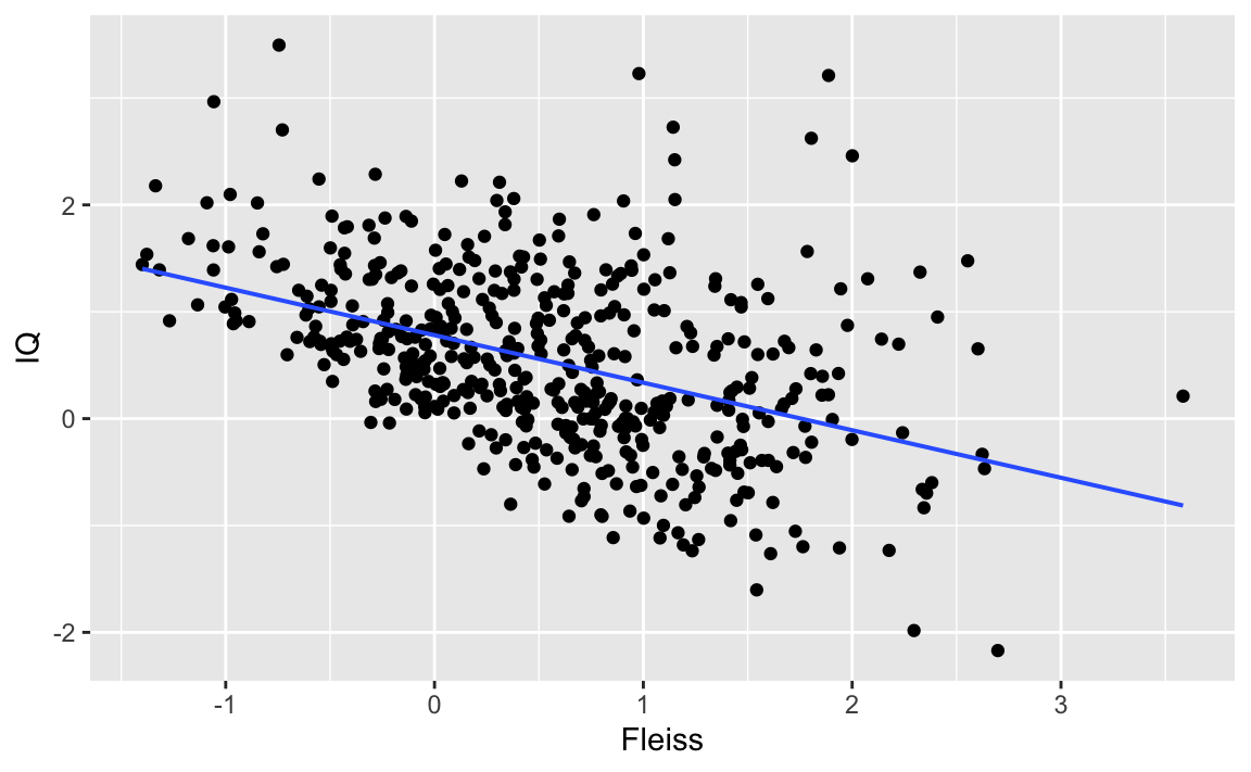

Replication effort: Second study provides conflicting evidence: No assocation between IQ and dilligence

A replication study, now endowed with an an larger (double) sample size, does not find any assocation. Noteworthy, they did not only include students, but non-students as well.

cor(IQ ~ Fleiss, data = df)
#> [1] 0.009981927

gf_point(IQ ~ Fleiss, data = df) %>% 
  gf_refine(scale_colour_colorblind())  %>% 
  gf_lm()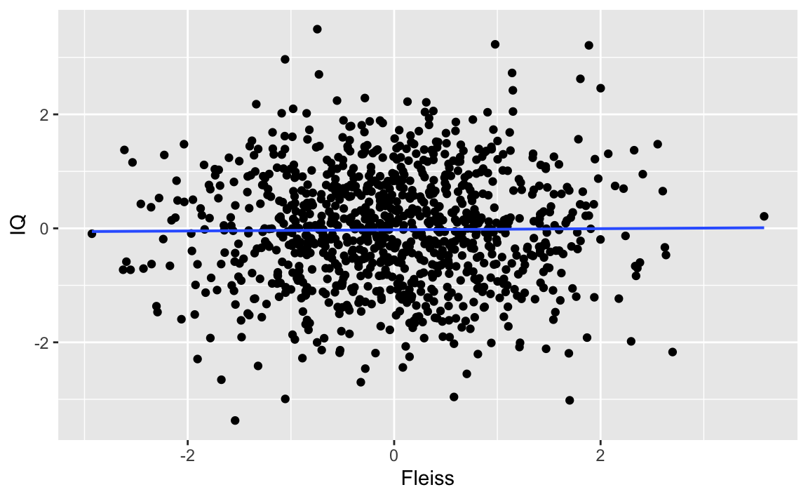

Stratifying subgroups

The seemingly paradox situation can be resolved once we stratify the larger (second) sample.

gf_point(IQ ~ Fleiss, color = ~Studium_bin, data = df) %>% 
  gf_refine(scale_colour_colorblind())  %>% 
  gf_refine(theme(legend.position = "bottom")) %>% 
  gf_labs(color = "") %>% 
  gf_lm()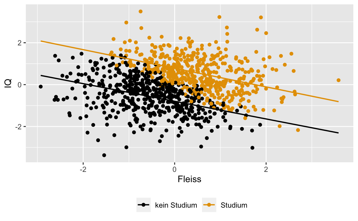

We see that there’s indeed a negative correlation in each subgroup. However, there’s no marginal assocation, ie., on the whole sample.

Causal interpretation

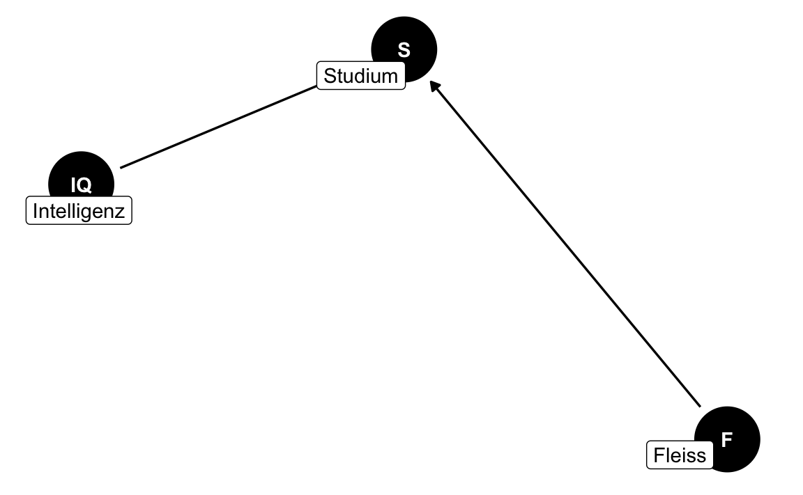
This pattern is called a collider bias in causal inference. The underlying causal structure can be visualizes using this DAG:

detach(name = "package:mosaic", unload = TRUE)
dag1 <- ggdag::dagify(S ~ F + IQ,
                      outcome = "S",
                      labels = c("S" = "Studium",
                                 "IQ" = "Intelligenz",
                                 "F" = "Fleiss"))

dag1_p <- ggdag(dag1, use_labels = "label")  + theme_dag_blank()

dag1_p