Load packages

library(tidyverse)
library(emojifont)
library(showtext)
library(ggpubr)

Pictogram waffle plot

A Pictogram may be defined as a (statistical) diagram using icons or similar “iconic” graphics to illstrate stuff. The waffle plot (see this post) is a nice object where to combine waffle and pictorgrams. Originally, this post was inspired by HRBRMSTR waffle package, see this post, but I could not get it running.

Maybe the easiest way is to work through an example (spoiler: see below for what we’re heading at).

Choose pictrograms

Say, we are looking for pictorgram related to persons. We can take advantage of the following functions to look up pictrogram from Font Awesome:

search_fontawesome("fa-person")
#> character(0)
search_fontawesome("fa-man")
#> character(0)

No luck; let’s check the cheatsheet of Font Awesome.

Note that we need to prefix fa- for the pictograms’ (also called “glyphs”) names.

The cheatsheet told me that this would work:

fa1 <- fontawesome(c("fa-user"))
fa2 <- fontawesome(c("fa-female", "fa-male"))

Font Awesome Free Licence

Free!

From the Licence Page:

Font Awesome Free is free, open source, and GPL friendly. You can use it for commercial projects, open source projects, or really almost whatever you want.

Icons — CC BY 4.0 License

In the Font Awesome Free download, the CC BY 4.0 license applies to all icons packaged as .svg and .js files types.

Fonts — SIL OFL 1.1 License

In the Font Awesome Free download, the SIL OFL license applies to all icons packaged as web and desktop font files.

Code — MIT License

In the Font Awesome Free download, the MIT license applies to all non-font and non-icon files.

Attribution

Attribution is required by MIT, SIL OFL, and CC BY licenses. Downloaded Font Awesome Free files already contain embedded comments with sufficient attribution, so you shouldn’t need to do anything additional when using these files normally.

We’ve kept attribution comments terse, so we ask that you do not actively work to remove them from files, especially code. They’re a great way for folks to learn about Font Awesome.

Make up some data

set.seed(42)
d <- crossing(x = 1:10,
              y = 1:10) %>%
  mutate(label = sample(x = c(rep(1, 20), rep(0, 80))) %>% as.factor()) %>%
  mutate(label2 = c(rep(1, 20), rep(0, 80)) %>% as.factor(),
         label3 = c(sample(x = c(rep(1, 10), rep(0, 40))),
                    sample(x = c(rep(1, 10), rep(0, 40)))),
         group = c(rep(fa2[1], 50), rep(fa2[2], 50))) %>%
  mutate(label3 = as.factor(label3),
         label4 = rep(1, 100) %>%
         as.factor())

That dataframe looks complex, but don’t worry, we’ll cover each part turn in turn.

Showtext

We will use the package showtext to render the icons. I found that this works well. Note that showtext renders text in a special way (see vignette for more details), and this rendering in not compatible (as to yet) to RStudio’s rendering. Just save the output to a file, or open a X11 or quartz window (depending on your operation system).

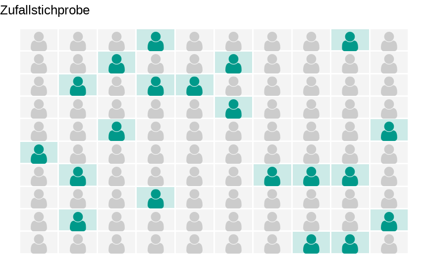
showtext_auto()

Plot 1

p1 <- ggplot(d, aes(x = x, y = y, color = label)) +
  geom_tile(color = "white", size = .5, aes(fill = label), alpha = .2) +
  theme_void() +
  geom_text(family='fontawesome-webfont', size=8, label = fa1) +
  scale_color_manual(label = c("nicht-gewählt", "gewählt"),
                     values = c("grey80", "#00998A"),
                     name = "") +
  scale_fill_manual( values = c("grey80", "#00998A"))+
  labs(title = "Zufallstichprobe") +
  theme(legend.position = "none") +
  guides(fill = FALSE)

p1

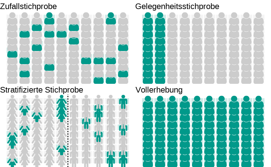
More similar plots

p2 <- ggplot(d, aes(x = x, y = y, color = label2)) +
  geom_tile(color = "white", size = .5, aes(fill = label2), alpha = .2) +
  theme_void() +
  geom_text(family='fontawesome-webfont', size = 8, label = fa1) +
  scale_color_manual(label = c("nicht-gewählt", "gewählt"),
                     values = c("grey80", "#00998A"),
                     name = "") +
  scale_fill_manual( values = c("grey80", "#00998A")) +
  labs(title = "Gelegenheitsstichprobe") +
  theme(legend.position = "none") +
  guides(fill = FALSE)

p3 <- ggplot(d, aes(x = x, y = y, color = label3)) +
  geom_tile(color = "white", size = .5, aes(fill = label3), alpha = .2) +
  theme_void() +
  geom_text(family='fontawesome-webfont', size = 8, aes(label = group)) +
  scale_color_manual(label = c("nicht-gewählt", "gewählt"),
                     values = c("grey80", "#00998A"),
                     name = "") +
  scale_fill_manual( values = c("grey80", "#00998A")) +
  labs(title = "Stratifizierte Stichprobe") +
  theme(legend.position = "none") +
  guides(fill = FALSE) +
  geom_vline(xintercept = 5.5, linetype = "dashed")


p4 <- ggplot(d, aes(x = x, y = y, color = label4)) +
  geom_tile(color = "white", size = .5, fill = "#00998A", alpha = .2) +
  theme_void() +
  geom_text(family='fontawesome-webfont', size = 8, label = fontawesome("fa-user")) +
  scale_color_manual(label = "gewählt",
                     values = "#00998A",
                     name = "") +
  scale_fill_manual(values = "#00998A") +
  labs(title = "Vollerhebung") +
  theme(legend.position = "none") +
  guides(fill = FALSE)

Plot altogether

ggarrange(p1, p2, p3, p4, nrow = 2, ncol = 2)

Debrief

To integrate emojifont to RMarkdown, checkout this post, along with its source code.

Pictogram waffle plot using emojifont