Load packages

library(tidyverse)
library(mosaic)

The Gaussian

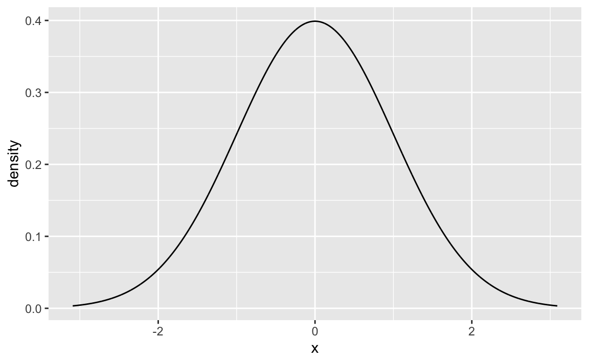
The ubiquituous Gaussian (aka normal) distribution is probably the most widely known distribution for stochastic process (although maybe as frequently encountered as a unicorn).

Here it is in all its glory.

gf_dist("norm")

There are two typical ways, why it may be considered “normal”, one is using the Galton Board, and one approach is building on the Central Limit Theorem. While such considerations are great for understanding “where” the Gaussian distribution comes from, this post explore some other direction of intuiton. Namely, how can one make sense of the formula of the Gaussian distribution?

Here is the density function of the Gaussian:

\[ f(x) = \frac{1}{\sqrt{2\pi \sigma^2}}e^{-\frac{(x-y)^2}{2\sigma^2}} \]

First Idea: Could the Gaussian be approximated via a linar function?

A linear function would be the most simple case. However an instant of thought tells us that this way is a dead end. A linear function has no maximum, but the Gaussian does have a maximum.

gf_abline(slope = 1, intercept = 0)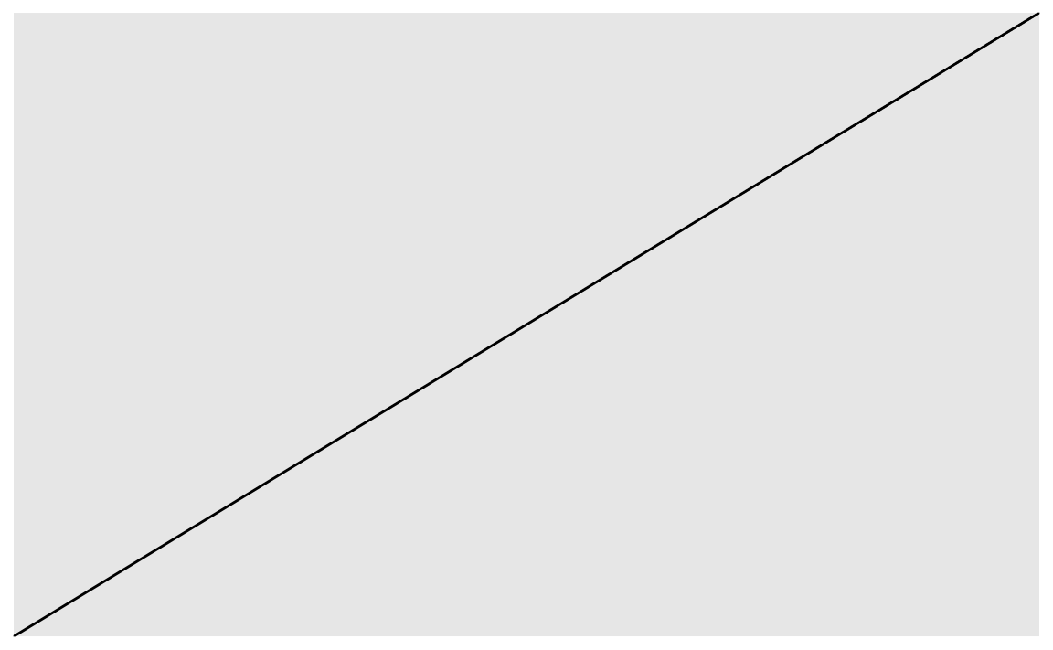

Does not work

Second Idea: A quadratic function can have a maximum

OK, a linear function does not have a maximum, but a quadratic function may have a maximum, as the Gaussian does. Maybe we can “re-engineer” the Gaussian by using some quadratic function? Let’s see.

f <- makeFun(-x^2 ~ x)

x <- seq(from = -5, to = 5, by = 0.1)
plotFun(f(x) ~ x)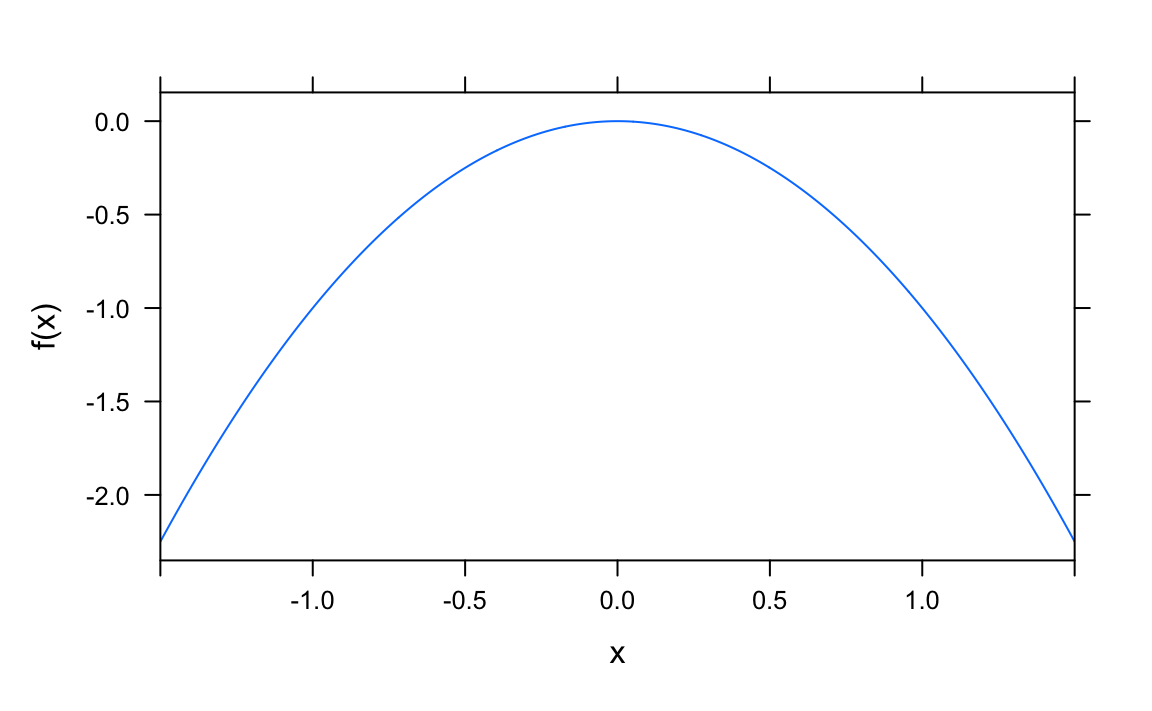

In ggplot2 terms:

p <- ggplot(data = data.frame(x = x), 
            mapping = aes(x = x))
p + stat_function(fun = f)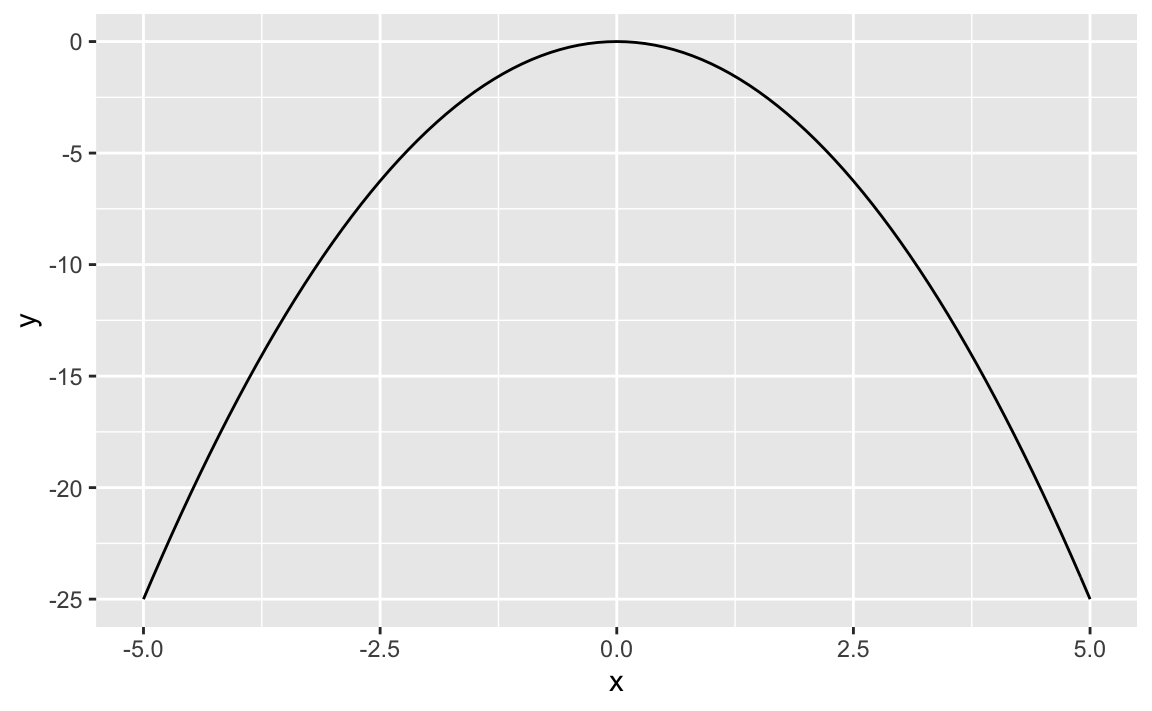

Better, but not really close to a normal distribution

Some function that yields large values for x’s close to zero…

We need some function that yields large (positive) values for x’s clos to zero (no matter whether we are approaching zero from left or right), and that yields small positive values for larger values (and increasingly so for even larger values).

Don’t worry about magnitudes (how large), we can try to standardize later (ie., divide by some value to adjust the absolute magnitude of our function.)

Hey, a quite simple function that fulfills this requirement is

\[ f(x) 2^{-x} \]

See:

x <- -5:5
y <- 2^-x^2
y
#>  [1] 2.980232e-08 1.525879e-05 1.953125e-03 6.250000e-02 5.000000e-01
#>  [6] 1.000000e+00 5.000000e-01 6.250000e-02 1.953125e-03 1.525879e-05
#> [11] 2.980232e-08

For any real number \(k\), we are sure to get a positive value if we plug \(k\) into \(k^-x^2\) for any real \(x\).

Let’s plot that.

f <- makeFun(2^(-x^2) ~ x)
#plotFun(f)
gf_function(fun = f, xlim = c(-5, 5))

In more simple R terms:

x <- seq(-5,5, .1)
y <- 2^(-x^2)

gf_line(y ~ x)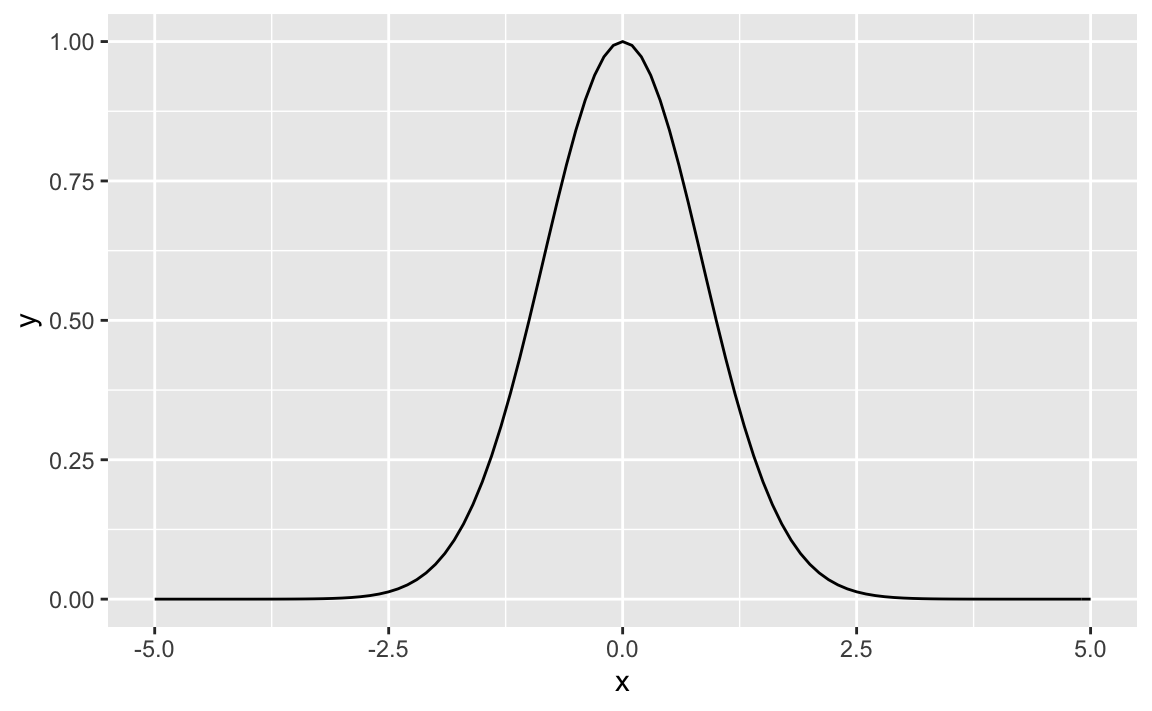

That looks great!

What about some other bases \(k\), such as 3?

f <- makeFun(3^(-x^2) ~ x)
gf_function(fun = f, xlim = c(-5, 5))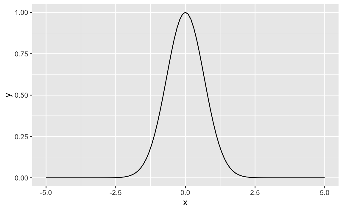

or \(k=100\)?

f <- makeFun(100^(-x^2) ~ x)
gf_function(fun = f, xlim = c(-5, 5))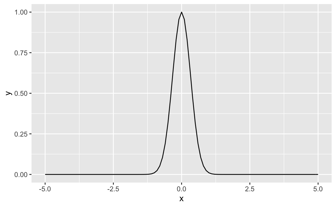

Well, the choice of the base \(k\) appears to make some difference, look at the spike. So, we are obviously close but not perfectly there, at the normal Gaussian.

Stop and pause

Our reengineering of the Gaussian is quite close, although not perfect. But we have covered a long way just using simple heuristics and intuition.

Comparing that with the Gaussian distribution formula above, note that the whole of the demoninator serves to standardize the area under the curve to 1.

Besides that we are nearly there: Let’s take 2.71 (or \(e\)) as our base, and we have found a Gaussian with some particular mean (0) and some SD.

f <- makeFun(2.71^(-x^2) ~ x)
gf_function(fun = f, 
            xlim = c(-3, 3))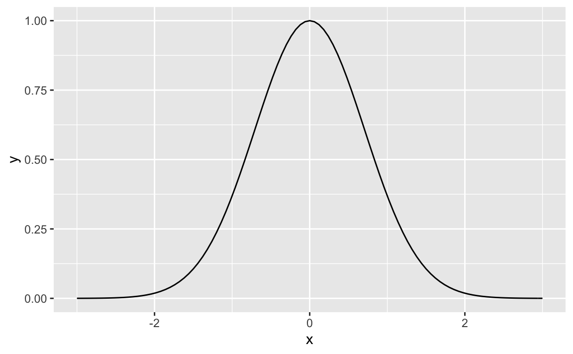

Compare to the Normal distribution

We have not adjusted the magnitudes (y axis), but besides, we appear to have found a pretty neat approximation of the Normal, just using basic, simple tools.

gf_dist("norm")