Load packages

library(tidyverse)  # data wrangling
library(mosaic)  # funplot
library(plotly)  # interactive plots
library(scatterplot3d)  # nomen est omen
library(rsm)  # 3d scatterplots

Motivation

Linear models are a standard way of predicting or explaining some data. Visualizing data is not only of didactical value but provides heuristical value too, as demonstrated by Anscombe’s Quartet.

Visualizing linear models in 2D is straightforward, but visualizing linear models with more than one predictor is much less so. The aim of this post is to demonstrate some ways do visualize linear models with more than one predictor, using popular R packages. We will focus on 3D examples, that is, two predictors.

Setup

Some data

data(mtcars)

Some packages

library(tidyverse)
library(mosaic)

Baseline model

For the sake of simplicity, let’s start with a 2D model.

lm0 <- lm(mpg ~ hp, data = mtcars)

`mosaic``

plotModel(lm0)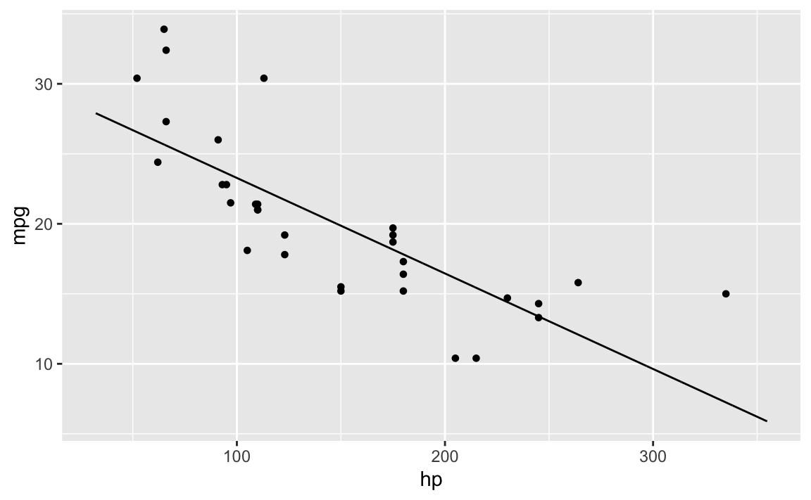

`ggformula``

gf_point(mpg ~ hp, data = mtcars) %>% 
  gf_lm()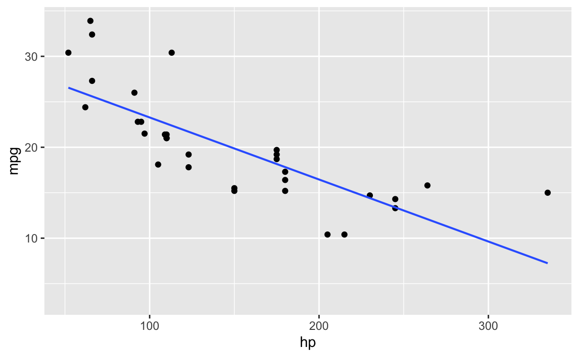

`ggplot2`

f0 <- function(x) {coef(lm0)[1] + coef(lm0)[2] * x}

ggplot(mtcars) +
  aes(x = hp, y = mpg) +
  geom_point() +
  stat_function(fun = f0)

`makeFun`

Extracting the function itself from a linear model can be achieved like this:

f0 <- makeFun(lm0)
f0
#> function (hp, ..., transformation = function (x) 
#> x) 
#> return(transformation(predict(model, newdata = data.frame(hp = hp), 
#>     ...)))
#> <environment: 0x7f8528a74eb0>
#> attr(,"coefficients")
#> (Intercept)          hp 
#> 30.09886054 -0.06822828

Then again:

ggplot(mtcars) +
  aes(x = hp, y = mpg) +
  geom_point() +
  stat_function(fun = f0)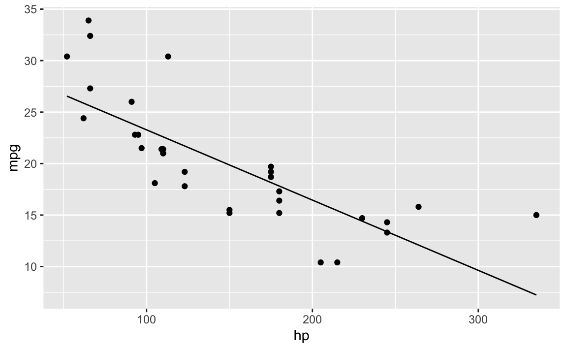

Our (initial) linear model for 3D

lm1 <- lm(mpg ~ hp * disp, data = mtcars)

Note that this notation is synonymous to this one:

lm1 <- lm(mpg ~ hp + disp + hp:disp, data = mtcars)

`gf_function_2d()`

Let’s briefly check the range of the predictors:

preds <- c("hp", "disp")

mtcars %>% 
  dplyr::select(one_of(preds)) %>% 
  summarise_all(funs(min, max))
#>   hp_min disp_min hp_max disp_max
#> 1     52     71.1    335      472

We’ll use this information to gauge the limits of the following graph:

f1 <- makeFun(lm1)

p1 <- gf_function_2d(f1, xlim = c(50, 300), ylim = c(50, 500)) %>% 
  gf_labs(x = "hp", y = "disp") %>% 
  gf_refine(scale_fill_viridis_c())
p1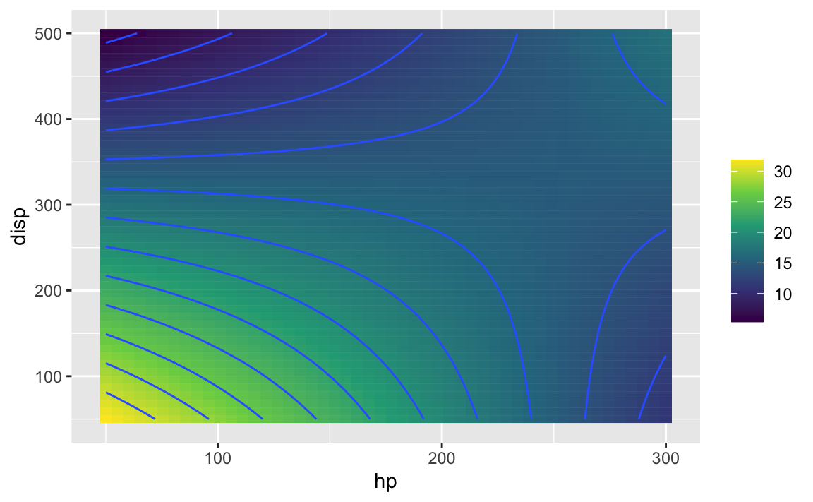

Computing a grid and plotting it

First we devise seom combinations of hp and disp values. Then we predict the mpg values based on those values using lm1.

hp_disp_grid <- expand_grid(hp = seq(50, 300, by = 10), disp = seq(50, 500, by= 10))


grid2 <- hp_disp_grid %>% 
  mutate(mpg_pred_lm1 = predict(lm1, newdata = data.frame(hp, disp)))

Check

gf_density(~mpg_pred_lm1, data = grid2)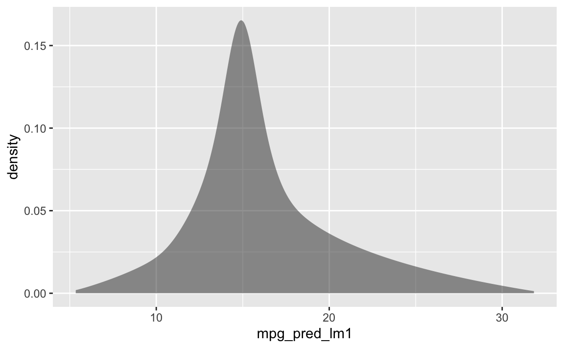

Now add the predicted value to the mtcars dataframe too:

mtcars <- mtcars %>% 
  mutate(pred_lm1 = predict(lm1))

ggplot(aes(x = hp, y = disp), data = grid2) +
  geom_raster(aes(fill = mpg_pred_lm1)) +
  scale_fill_viridis_c() +
  geom_point(data = mtcars, aes(color = pred_lm1)) +
  scale_color_viridis_c()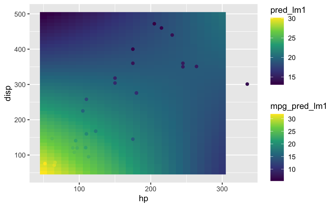

`plotFun` as tile plot (heatmap)

mosaic provides a convenient function to plot linear models with predictors, plotFun().

plotFun(f1(hp, disp) ~ hp & disp)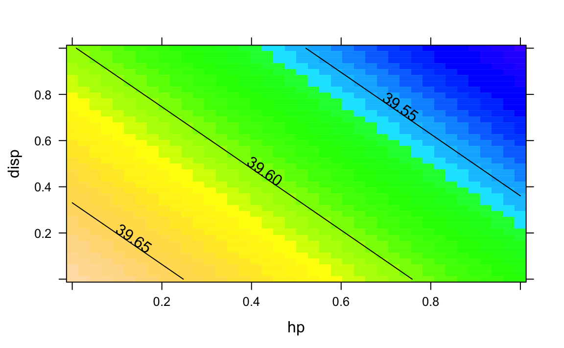

`plotFun` as 3d surface plot

plotFun(f1(hp, disp) ~ hp & disp, surface = TRUE)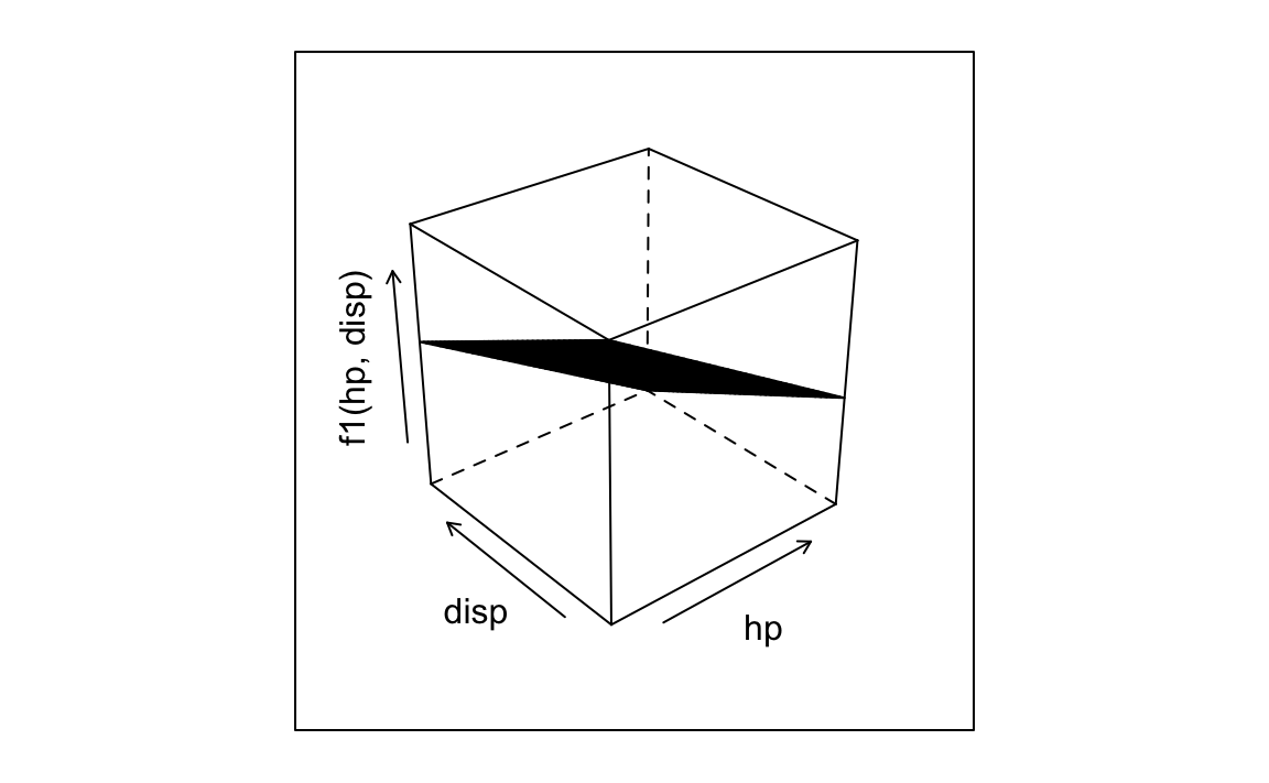

Plotly surface

For plotly surface, we need the data in wide format, ie., we need to spread them out, from long (tidy, standard) format to the wide format. In addition, there should be no more name (key) column, and it ought to be a matrix:

grid_wide <- grid2 %>% 
  pivot_wider(names_from = disp, values_from = mpg_pred_lm1) %>% 
  select(-1) %>% 
  as.matrix


rownames(grid_wide) <- seq(50, 300, by = 10)

xaxis <- list(
  title = "hp"
  #range = c(50, 300)
)

yaxis <- list(
  title = "disp"
  #range = c(50, 500)
)

zaxis <- list(
  title = "mpg"
  #range = c(10, 30)
)

p <- plot_ly(z = ~grid_wide, 
             x = seq(50, 300, by = 10),
             y = seq(50, 500, by = 10)) %>% 
  add_surface(
  contours = list(
    z = list(
      show=TRUE,
      usecolormap=TRUE,
      highlightcolor="#ff0000"
      #project=list(z=TRUE)
      )
    )
  ) %>%
    layout(
    title = "lm1 as 3d plane",
    scene = list(
      xaxis = xaxis,
      yaxis = yaxis,
      zaxis = zaxis
    ))

p

`persp()`

x <- seq(min(mtcars$hp), max(mtcars$hp), length.out = 25)
y <- seq(min(mtcars$disp), max(mtcars$disp), length.out = 25)
z <- outer(x, y, function(x,y) {predict(lm1, data.frame(hp = x, disp = y))})
persp(x,y,z , theta = c(45, 135, 225, 315), col = "lightblue")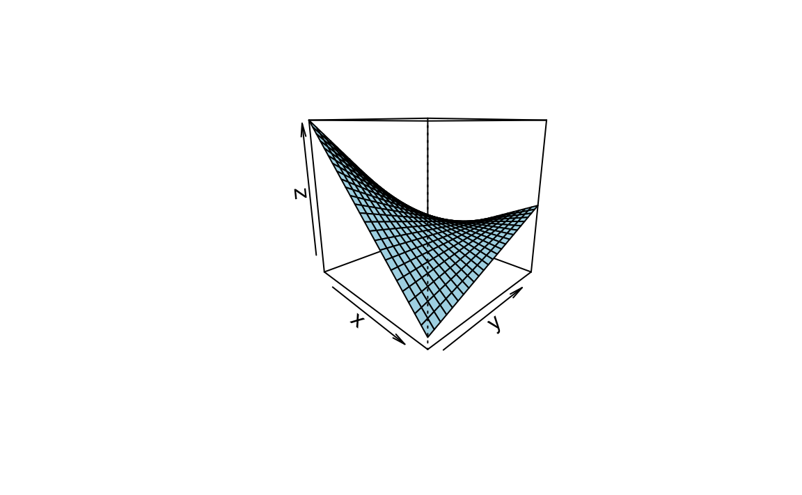

`contour()`

From package rsm we can make use of contour():

contour(lm1, hp ~ disp, image = TRUE)
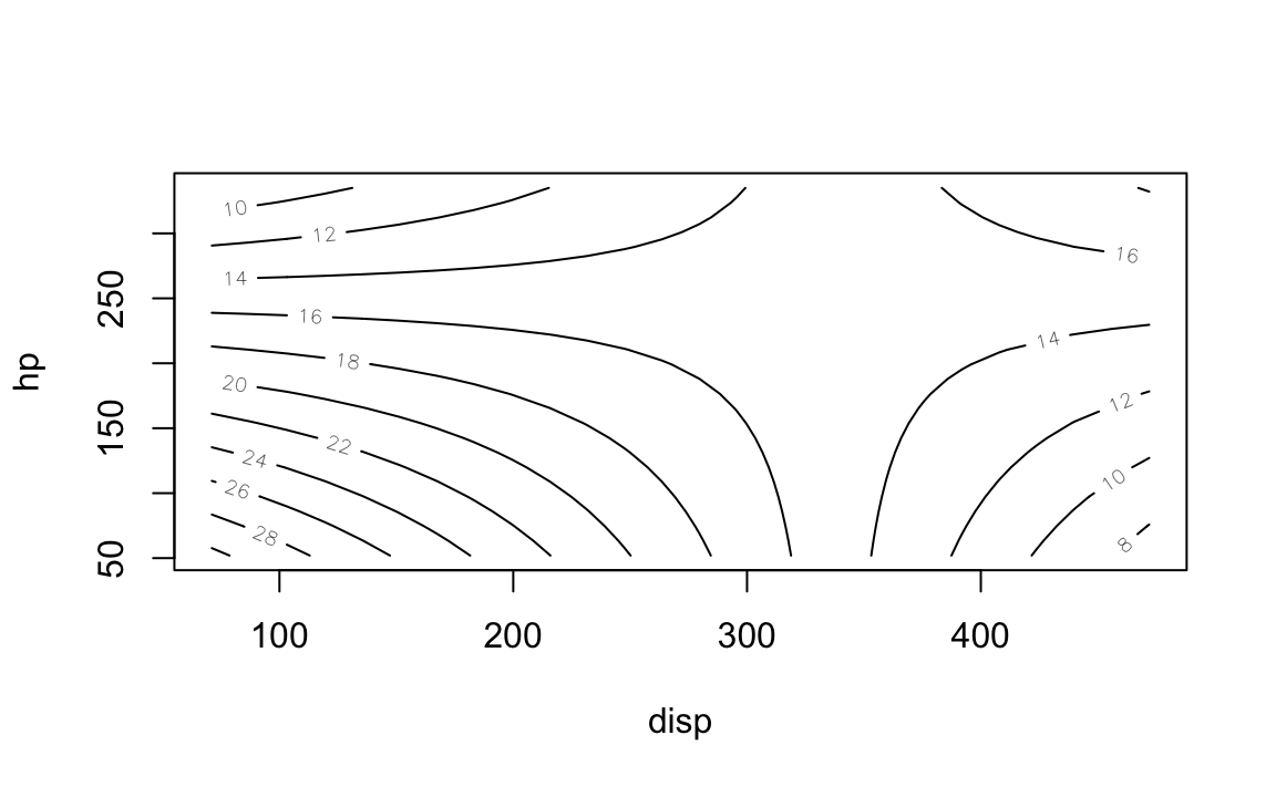
contour(lm1, hp ~ disp, image = FALSE)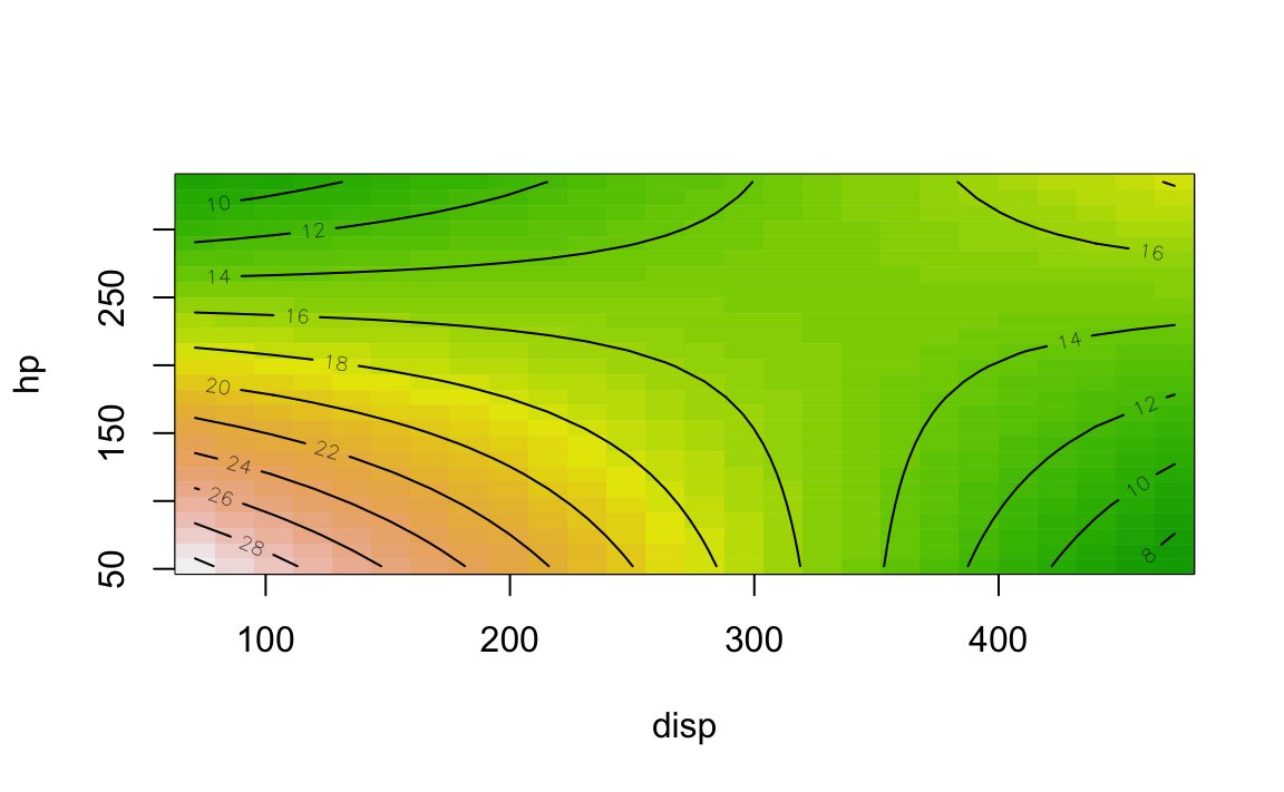

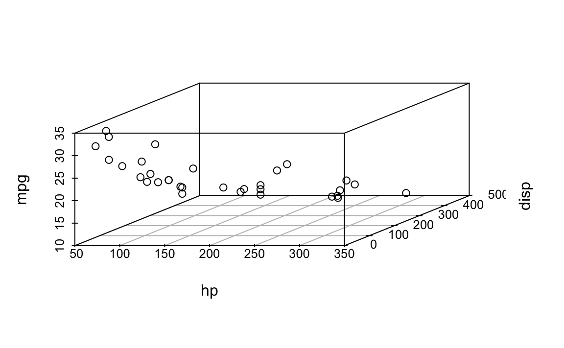
Scatterplot 3d

First plot the scatterplot:

d <- mtcars %>% 
  select(hp, disp, mpg)
lm1a <- lm(d$mpg ~ d$hp + d$disp)



p3 <- scatterplot3d(d)

Now add the regression plane:

p3$plane3d(lm1a)
#> Error in segments(x, z1, x + y.max * yx.f, z2 + yz.f * y.max, lty = ltya, : plot.new has not been called yet

For some reason, this code does not run in (my) rmarkdown setup, but it worked (on my machine) in a ordinary R script.

Some ways for plotting 3D linear models