Load packages

library(tidyverse)
library(mosaic)

Motivation

The p-value is a ubiquituous tool for gauging the plausibility of a Null hypothesis. More specifically, the p-values indicates the probability of obtaining a test statistic at least as extreme as in the present data if the Null hypothesis was true and the experiment would be repeated an infinite number of times (under the same conditions except the data generating process).

The distribution of the p-values depends on the strength of some effect (among other things). The bigger the effect, the smaller the p-values (ceteris paribus). In the extreme, if the effect is zero, that is, if the Null is true, the distribution will be equally spread out. As this sounds not overly intuitive maybe, let’s simulate it.

There are of course nice proofs out there, this one is quite straigt forward for example.

Simulate p-values for the Null

Let our experiment consist of a t-test with two groups of n=30, and the Null being true. Further, let the distribution be standard normal. We’ll test two-sided, and take an alpha of .05 for granted.

Let’s simply extract the p-value:

get_p_from_ttest_sim <- function(n = 30, my_m = 0, my_sd = 1) {
  
  sample1 <- rnorm(n = n, mean = my_m, sd = my_sd) 
  sample2 <- rnorm(n = n, mean = my_m, sd = my_sd)  
  
  p <- t.test(x = sample1, y = sample2)$p.value
  
  p <- list(p_value = p)
  
  return( p)
}

Test it:

get_p_from_ttest_sim()
#> $p_value
#> [1] 0.9270056

Now rerun this simulated experiment a couple of times:

k <- 1e05
ps <- do(k) * get_p_from_ttest_sim()

Plot it

gf_histogram(~p_value, data = ps, bins = 10)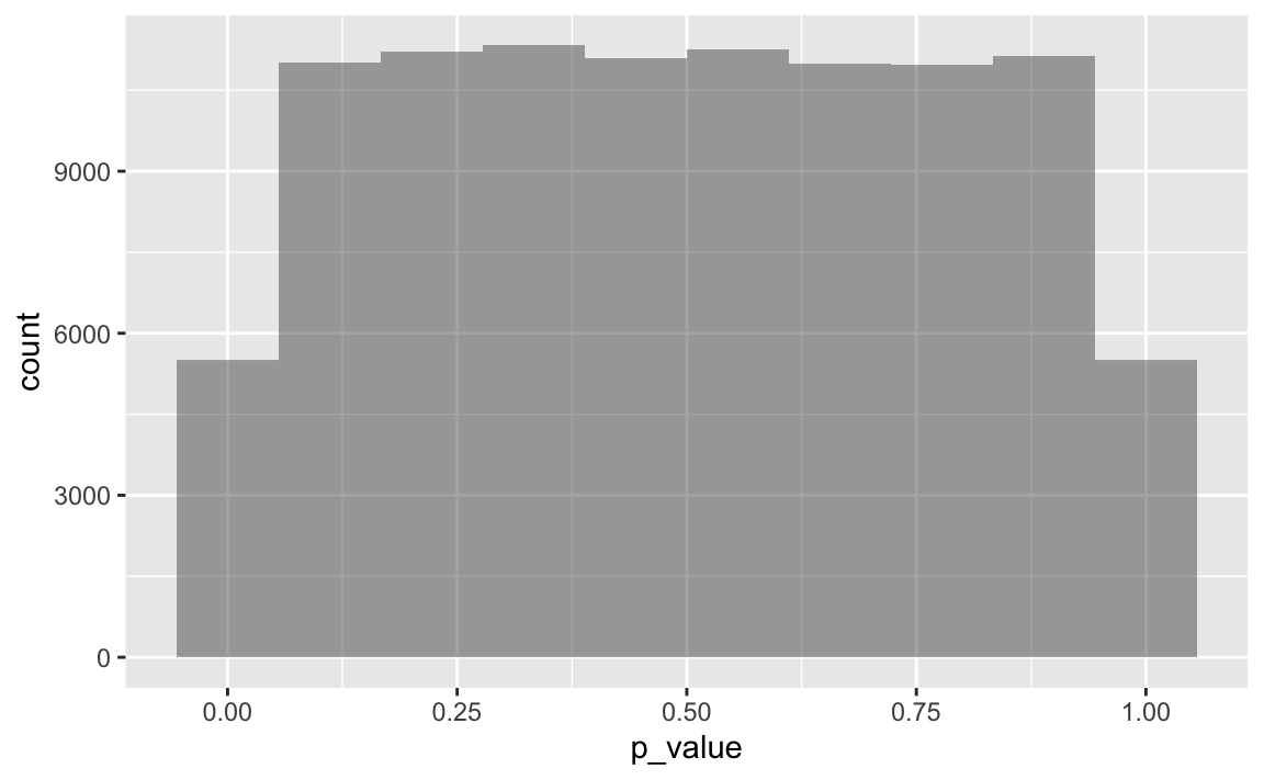

Closer look

Let’s compute the proportion of significant p-values, ie p<.05. That should sum up to approx. 5%.

ps %>% 
  filter(p_value < .05) %>% 
  summarise(p_prop = n()/k)
#>   p_prop
#> 1 0.0491

And now let’s cut the range in 10 bins:

ps %>% 
  mutate(bins = cut(p_value, breaks = 11)) %>% 
  group_by(bins) %>% 
  summarise(p_prop = n())
#> # A tibble: 11 x 2
#>    bins              p_prop
#>    <fct>              <int>
#>  1 (-0.00098,0.0909]   8989
#>  2 (0.0909,0.182]      9028
#>  3 (0.182,0.273]       9225
#>  4 (0.273,0.364]       9247
#>  5 (0.364,0.455]       9143
#>  6 (0.455,0.545]       9137
#>  7 (0.545,0.636]       9192
#>  8 (0.636,0.727]       8948
#>  9 (0.727,0.818]       8918
#> 10 (0.818,0.909]       9121
#> 11 (0.909,1]           9052

Approximately identical group sizes.

Finally, let’s check the lower p-values to see if they are also uniformly distributed. Note that we reduce the sample size greatly by filtering on a small part of p-values so we should expect more variation around the expected value.

ps %>% 
  filter(p_value <= .05) %>% 
  mutate(bins =cut(p_value, breaks = 11)) %>% 
  group_by(bins) %>% 
  summarise(p_prop = n())
#> # A tibble: 11 x 2
#>    bins                p_prop
#>    <fct>                <int>
#>  1 (-3.02e-05,0.00456]    427
#>  2 (0.00456,0.00911]      450
#>  3 (0.00911,0.0136]       457
#>  4 (0.0136,0.0182]        465
#>  5 (0.0182,0.0227]        456
#>  6 (0.0227,0.0273]        462
#>  7 (0.0273,0.0318]        446
#>  8 (0.0318,0.0364]        432
#>  9 (0.0364,0.0409]        446
#> 10 (0.0409,0.0454]        432
#> 11 (0.0454,0.05]          437

As said there appears to be quite some variation within these bins.

And even more close-up:

ps %>% 
  filter(p_value <= .005) %>% 
  mutate(bins =cut(p_value, breaks = 11)) %>% 
  group_by(bins) %>% 
  summarise(p_prop = n())
#> # A tibble: 11 x 2
#>    bins                p_prop
#>    <fct>                <int>
#>  1 (1.48e-05,0.000471]     42
#>  2 (0.000471,0.000922]     41
#>  3 (0.000922,0.00137]      44
#>  4 (0.00137,0.00183]       40
#>  5 (0.00183,0.00228]       45
#>  6 (0.00228,0.00273]       38
#>  7 (0.00273,0.00318]       37
#>  8 (0.00318,0.00363]       48
#>  9 (0.00363,0.00408]       52
#> 10 (0.00408,0.00453]       39
#> 11 (0.00453,0.00499]       44