Reducing residual variance in modeling

Modeling is a central part not only of statistical inquiry, but also of everyday human sense-making. We use models as metaphors for the world, in a broader sense. Of course, a model that explains the world better (than some other model) is to be preferred, all other things being equal. In this post, we demonstrate that a more “clever” statistical model reduces the residual variance. It should be noted that this “noise reduction” comes at a cost, however: The model gets more complex; there a more parameters in the model.

First, let’s load some data and usual packages:

library(tidyverse)
library(mosaic)
library(gridExtra)

data(tips, package = "reshape2")

We filter only the extreme groups in order to carve out the effect more lucidly. In addition, let’s compute the residuals and the square residuals:

tips2 <- filter(tips, size %in% c(1, 6)) %>% 
  mutate(ID = 1:nrow(.),
         tip_resid = tip - mean(tip),
         tips_resid_quad =tip_resid^2) %>% 
  group_by(size) %>% 
  mutate(tip_mean_group = mean(tip))

glimpse(tips2)

## Rows: 8
## Columns: 11
## Groups: size [2]
## $ total_bill      <dbl> 3.07, 10.07, 7.25, 29.80, 34.30, 27.05, 48.17, 8.58
## $ tip             <dbl> 1.00, 1.83, 1.00, 4.20, 6.70, 5.00, 5.00, 1.92
## $ sex             <fct> Female, Female, Female, Female, Male, Female, Male, Ma…
## $ smoker          <fct> Yes, No, No, No, No, No, No, Yes
## $ day             <fct> Sat, Thur, Sat, Thur, Thur, Thur, Sun, Fri
## $ time            <fct> Dinner, Lunch, Dinner, Lunch, Lunch, Lunch, Dinner, Lu…
## $ size            <int> 1, 1, 1, 6, 6, 6, 6, 1
## $ ID              <int> 1, 2, 3, 4, 5, 6, 7, 8
## $ tip_resid       <dbl> -2.33125, -1.50125, -2.33125, 0.86875, 3.36875, 1.6687…
## $ tips_resid_quad <dbl> 5.4347266, 2.2537516, 5.4347266, 0.7547266, 11.3484766…
## $ tip_mean_group  <dbl> 1.4375, 1.4375, 1.4375, 5.2250, 5.2250, 5.2250, 5.2250…

tip_mean_group refers to the mean value of the response variable tip for each conditioned group.

Next, we compute a helper data frame that stores the group means only:

tips_sum <- tips2 %>% 
  group_by(size) %>% 
  summarise(tip = mean(tip))

Now, let’s plot:

That’s the plot for the simpler model without consideration of subgroups. We model the target variable tip as the grand mean (of the whole data set).

p2 <- ggplot(tips2) +
  geom_hline(aes(yintercept = mean(tip))) +
  geom_segment(aes(x = ID,
                   xend = ID,
                   y = tip,
                   yend = mean(tip)),
               color = "grey80") +
  geom_point(aes(x = ID, y = tip)) +
  labs(title = "tip ~ 1")
p2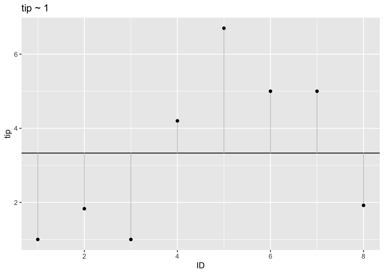

In contrast, consider the residuals when conditioned on the subgroup means:

p1 <- ggplot(tips2) +
  geom_hline(data = tips_sum,
            aes(yintercept = tip,
                color = factor(size))) +
  geom_segment(aes(x = ID,
                   xend = ID,
                   y = tip,
                   yend = tip_mean_group),
               color = "grey80") +
  geom_point(aes(x = ID, y = tip,
                 color = factor(size))) +
  theme(legend.position = "none") +
  labs(title = "tip ~ size")
p1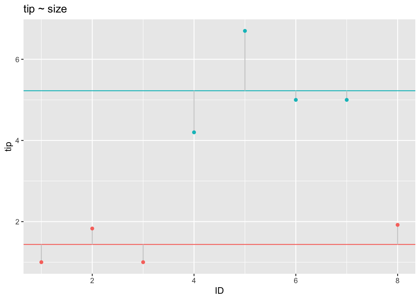

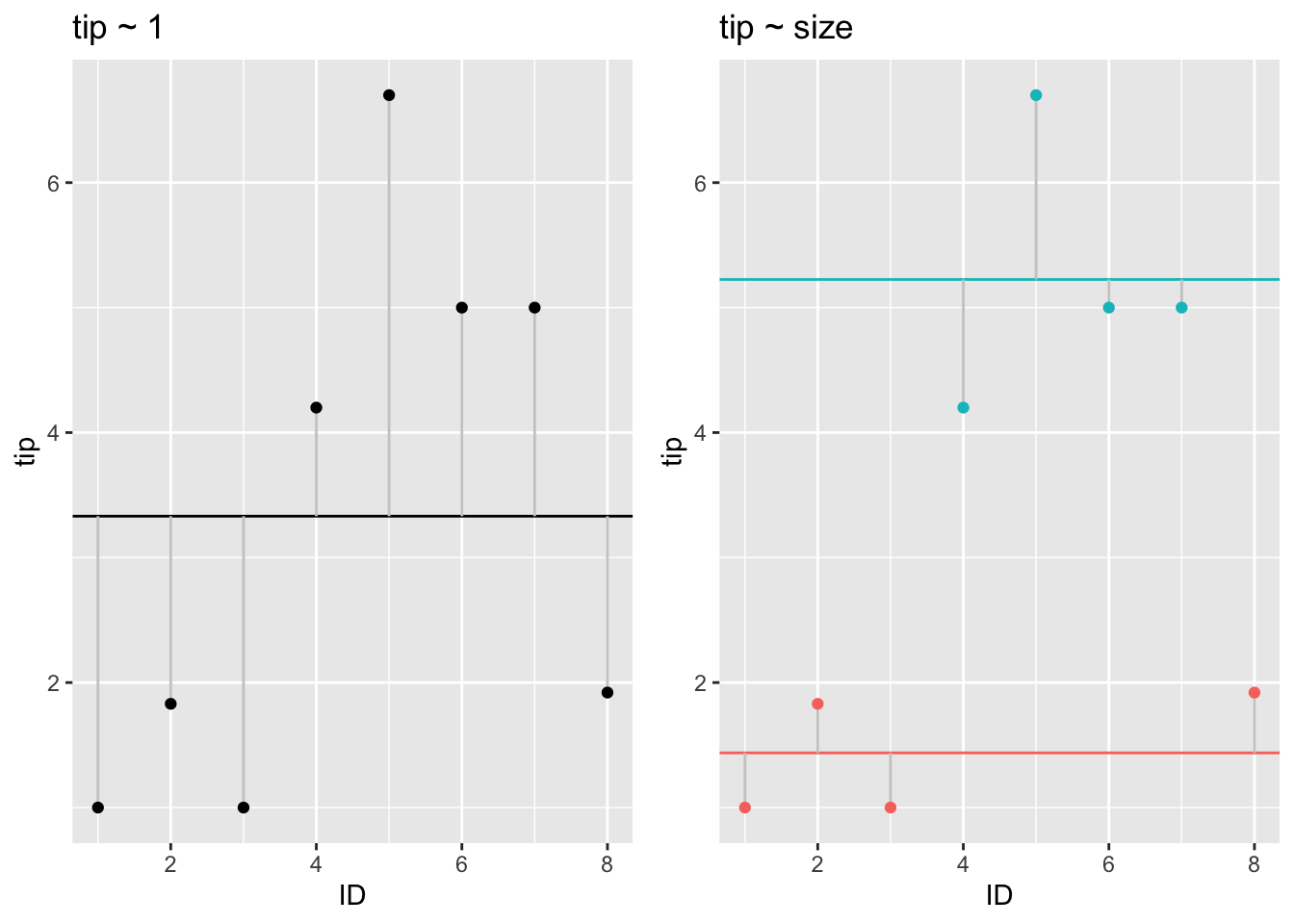
As can be seen, the residuals become smaller in this model: The more complex model, where the target variable is modeled as the subgroup average, explains the data better. This models shows a better fit to the data.

grid.arrange(p2, p1, nrow = 1)