A typical “cook book recipe” for doing data analysis is an applied stats course is:
- report descriptive statistics
- plot some nice diagrams
- test hypothesis
- report effect sizes
Let’s have a quick glance at these steps. We will use the dataset flights of the package nycflights13.
data(flights, package = "nycflights13")This post will be tidyverse-driven.
library(tidyverse)
library(skimr)
library(mosaic)
Let’s compute some summaries:
flights %>%
  select(arr_delay) %>%
skim| Name | Piped data |
| Number of rows | 336776 |
| Number of columns | 1 |
| _______________________ | |
| Column type frequency: | |
| numeric | 1 |
| ________________________ | |
| Group variables | None |
Variable type: numeric
| skim_variable | n_missing | complete_rate | mean | sd | p0 | p25 | p50 | p75 | p100 | hist |
|---|---|---|---|---|---|---|---|---|---|---|
| arr_delay | 9430 | 0.97 | 6.9 | 44.63 | -86 | -17 | -5 | 14 | 1272 | ▇▁▁▁▁ |
Alternatively, using mosaic:
mosaic::favstats(~arr_delay, data = flights)| min | Q1 | median | Q3 | max | mean | sd | n | missing |
|---|---|---|---|---|---|---|---|---|
| -86 | -17 | -5 | 14 | 1.27e+03 | 6.9 | 44.6 | 327346 | 9430 |
Subgroup statistics
Differentiating between origin levels:
flights %>%
  select(arr_delay, origin) %>%
  group_by(origin) %>%
skim| Name | Piped data |
| Number of rows | 336776 |
| Number of columns | 2 |
| _______________________ | |
| Column type frequency: | |
| numeric | 1 |
| ________________________ | |
| Group variables | origin |
Variable type: numeric
| skim_variable | origin | n_missing | complete_rate | mean | sd | p0 | p25 | p50 | p75 | p100 | hist |
|---|---|---|---|---|---|---|---|---|---|---|---|
| arr_delay | EWR | 3708 | 0.97 | 9.11 | 45.53 | -86 | -16 | -4 | 16 | 1109 | ▇▁▁▁▁ |
| arr_delay | JFK | 2200 | 0.98 | 5.55 | 44.28 | -79 | -18 | -6 | 13 | 1272 | ▇▁▁▁▁ |
| arr_delay | LGA | 3522 | 0.97 | 5.78 | 43.86 | -68 | -17 | -5 | 12 | 915 | ▇▁▁▁▁ |
Alternatively, using mosaic:
favstats(arr_delay~origin, data = flights)| origin | min | Q1 | median | Q3 | max | mean | sd | n | missing |
|---|---|---|---|---|---|---|---|---|---|
| EWR | -86 | -16 | -4 | 16 | 1.11e+03 | 9.11 | 45.5 | 117127 | 3708 |
| JFK | -79 | -18 | -6 | 13 | 1.27e+03 | 5.55 | 44.3 | 109079 | 2200 |
| LGA | -68 | -17 | -5 | 12 | 915 | 5.78 | 43.9 | 101140 | 3522 |
Effect sizes
Cohen’s d
library(effsize)We need two groups not three:
flights2 <-
  filter(flights, origin != "JFK") %>%
  sample_n(1000) %>%
  na.omit
cohen.d(d = flights2$arr_delay,
f = flights2$origin)
#>
#> Cohen's d
#>
#> d estimate: 0.223211 (small)
#> 95 percent confidence interval:
#> lower upper
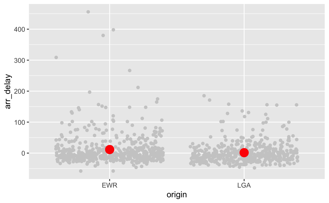
#> 0.0961037 0.3503182Plot mean difference
ggplot(flights2) +
  aes(x = origin, y = arr_delay) +
  geom_point(color = "grey80", position = "jitter") +
  stat_summary(fun.y = mean, geom = "point", color = "red", size = 5)
Other effect sizes
Other effect sizes can quite conveniently be derived from the package compute.es.