What this post is about: Data cleansing in practice with R
Data analysis, in practice, consists typically of some different steps which can be subsumed as “preparing data” and “model data” (not considering communication here):
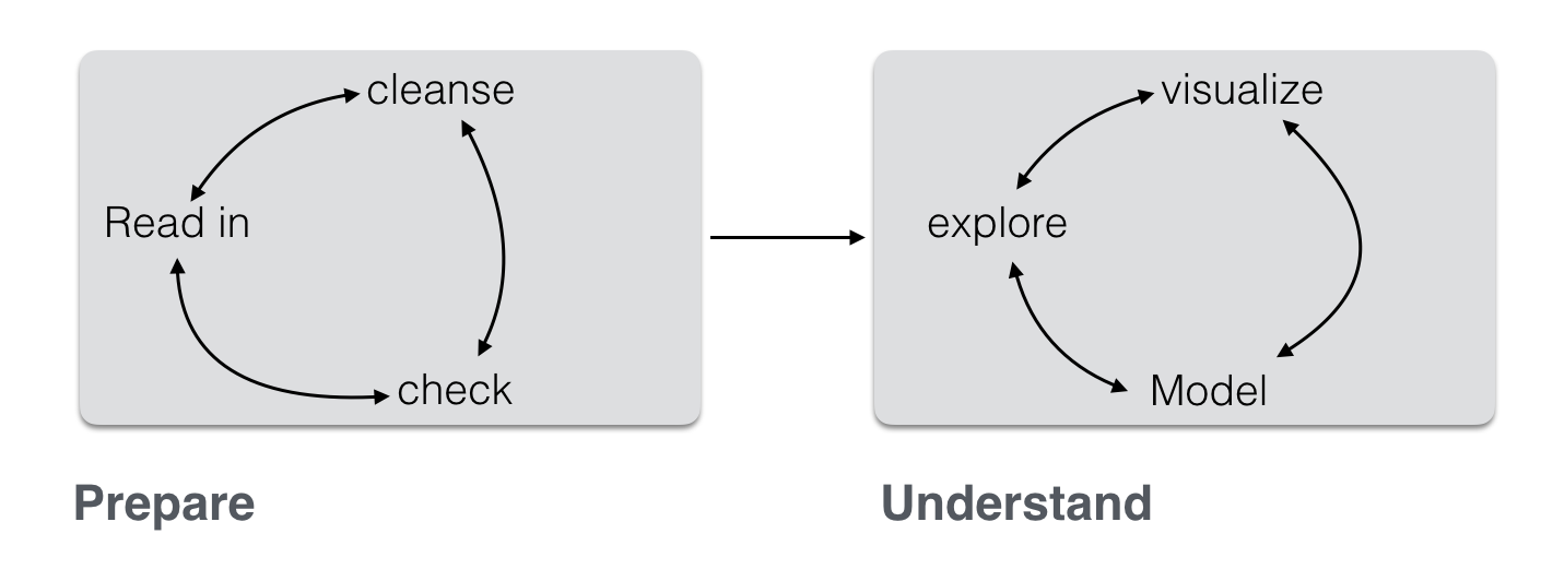
(Inspired by this)
Often, the first major part – “prepare” – is the most time consuming. This can be lamented since many analysts prefer the cool modeling aspects (since I want to show my math!). In practice, one rather has to get his (her) hands dirt…
In this post, I want to put together some kind of checklist of frequent steps in data preparation. More precisely, I would like to detail some typical steps in “cleansing” your data. Such steps include:
- identify missings
- identify outliers
- check for overall plausibility and errors (e.g, typos)
- identify highly correlated variables
- identify variables with (nearly) no variance
- identify variables with strange names or values
- check variable classes (eg. characters vs factors)
- remove/transform some variables (maybe your model does not like categorial variables)
- rename some variables or values (especially interesting if large number)
- check some overall pattern (statistical/ numerical summaries)
- center/scale variables
Don’t get lost in big projects
Before we get in some details, let’s consider some overall guidelines. I have noticed that some projects keep growing like weed, and I find myself bewildered in some jungle… The difficulties then arise not because data or models are difficult, but due to the sheer volume of the analysis.
All in a function
Put analytical steps which belong together in one function. For example, build one function for data cleansing, give as input the raw data frame and let it spit out the processed data frame after all your cleansing steps:
cleansed_data <- cleanse_data(raw_dirty_data,
                              step_01 = TRUE,
                              step_02 = TRUE,
                              step_03 = TRUE)
Although functions are a bit more difficult to debug, at the end of the day it is much easier. Normally or often the steps will be run many times (for different reasons), so it is much easier if all is under one roof.
That said, pragmtic programming suggests to start easy, and to refactor frequently. So better start with a simple solution that works than to have a enormous code that chokes. Get the code running, then improve on it.
Data set for practice
The OKCupid Data set (sanitized version, no names!) is quite nice. You can download it here.
In the following, I will assume that these data are available.
data(profiles, package = "okcupiddata")
data <- profiles
So, the data set is quite huge: 59946, 22 (rows/cols)
Let’s have a brief look at the data.
library(dplyr)
glimpse(data)
## Observations: 59,946
## Variables: 22
## $ age         <int> 22, 35, 38, 23, 29, 29, 32, 31, 24, 37, 35, 28, 24...
## $ body_type   <chr> "a little extra", "average", "thin", "thin", "athl...
## $ diet        <chr> "strictly anything", "mostly other", "anything", "...
## $ drinks      <chr> "socially", "often", "socially", "socially", "soci...
## $ drugs       <chr> "never", "sometimes", NA, NA, "never", NA, "never"...
## $ education   <chr> "working on college/university", "working on space...
## $ ethnicity   <chr> "asian, white", "white", NA, "white", "asian, blac...
## $ height      <int> 75, 70, 68, 71, 66, 67, 65, 65, 67, 65, 70, 72, 72...
## $ income      <int> NA, 80000, NA, 20000, NA, NA, NA, NA, NA, NA, NA, ...
## $ job         <chr> "transportation", "hospitality / travel", NA, "stu...
## $ last_online <dttm> 2012-06-28 20:30:00, 2012-06-29 21:41:00, 2012-06...
## $ location    <chr> "south san francisco, california", "oakland, calif...
## $ offspring   <chr> "doesn't have kids, but might want them", "doesn't...
## $ orientation <chr> "straight", "straight", "straight", "straight", "s...
## $ pets        <chr> "likes dogs and likes cats", "likes dogs and likes...
## $ religion    <chr> "agnosticism and very serious about it", "agnostic...
## $ sex         <chr> "m", "m", "m", "m", "m", "m", "f", "f", "f", "m", ...
## $ sign        <chr> "gemini", "cancer", "pisces but it doesn't matter"...
## $ smokes      <chr> "sometimes", "no", "no", "no", "no", "no", NA, "no...
## $ speaks      <chr> "english", "english (fluently), spanish (poorly), ...
## $ status      <chr> "single", "single", "available", "single", "single...
## $ essay0      <chr> "about me:    i would love to think that i was som...
What’s in a name?
With the code getting longer, it is easy to get confused about naming: data_v2_no_missings_collapsed is the right data matrix to proceed, wasn’t it? Or rather data_dat_edit_noNA_v3? Probably a helpful (though partial) solution is to prevent typing a lot. “Don’t repeat yourself” - if stuff is put inside a function, the objects will not clutter your environment, and you don’t have to deal with them all the time. Also, you will reduce code, and the number of objects if stuff is put inside functions and loops.
That raises the question who to name the data set? At least two points are worth thinking. First, the “root” name should it be the name of the project such as “OKCupid” or “nycflights13”? Or just something like “data”? Personally, I prefer “data” as it is short and everybody will know what’s going on. Second question: Should some data manipulations should be visible in the name of the object? I, personally, like this and do that frequently, eg., carat_mean, so I will remember that the mean is in there. However, for bigger projects I have made the experience that I lose track on which is the most recent version. So better do not put data manipulations in the name of the data frame. However, what one can do is use attributes, eg.:
data_backup <- removing_missings_somehow(data)  # pseudo funtion here for illustration
data <- data_backup

attr(data, "NA_status") <- "no_NA"
Checklist
Clearly, there are different ways to get to Rome; I present just one, which has proved helpful for me.
Identify missings
A key point is here to address many columns in one go, otherwise it gets laborious with large data sets. Here’s one way:
library(knitr)

data %>%
  summarise_all(funs(sum(is.na(.)))) %>% kable
| age | body_type | diet | drinks | drugs | education | ethnicity | height | income | job | last_online | location | offspring | orientation | pets | religion | sex | sign | smokes | speaks | status | essay0 |
|---|---|---|---|---|---|---|---|---|---|---|---|---|---|---|---|---|---|---|---|---|---|
| 0 | 5296 | 24395 | 2985 | 14080 | 6628 | 5680 | 3 | 48442 | 8198 | 0 | 0 | 35561 | 0 | 19921 | 20226 | 0 | 11056 | 5512 | 50 | 0 | 5485 |
The function kable prints a html table (package knitr).
There seem to be quite a bit missings. Maybe better plot it.
library(ggplot2)
library(tidyr)

data %>%
  summarise_all(funs(sum(is.na(.)))) %>%
  gather %>%
  ggplot(aes(x = reorder(key, value), y = value)) + geom_bar(stat = "identity") +
  coord_flip() +
  xlab("variable") +
  ylab("Absolute number of missings")
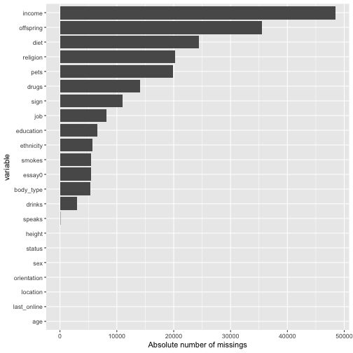
With this large number of missings, we probably will not find an easy solution. Skipping cases will hurt, but imputating may also not be appropriate. Ah, now I know: Let’s just leave it as it is for the moment :-)
Or, at least let’s remember which columns have more than, say, 10%, missings:
cols_with_some_NA <- round(colMeans(is.na(data)),2)
cols_with_too_many_NA <- cols_with_some_NA[cols_with_some_NA > .1]

# alterntively:
data %>%
  select_if(function(col) mean(is.na(col)) < .1) %>%
  head
##   age      body_type   drinks           ethnicity height
## 1  22 a little extra socially        asian, white     75
## 2  35        average    often               white     70
## 3  38           thin socially                <NA>     68
## 4  23           thin socially               white     71
## 5  29       athletic socially asian, black, other     66
## 6  29        average socially               white     67
##           last_online                        location orientation sex
## 1 2012-06-28 20:30:00 south san francisco, california    straight   m
## 2 2012-06-29 21:41:00             oakland, california    straight   m
## 3 2012-06-27 09:10:00       san francisco, california    straight   m
## 4 2012-06-28 14:22:00            berkeley, california    straight   m
## 5 2012-06-27 21:26:00       san francisco, california    straight   m
## 6 2012-06-29 19:18:00       san francisco, california    straight   m
##      smokes                                                speaks
## 1 sometimes                                               english
## 2        no english (fluently), spanish (poorly), french (poorly)
## 3        no                                  english, french, c++
## 4        no                              english, german (poorly)
## 5        no                                               english
## 6        no                    english (fluently), chinese (okay)
##      status
## 1    single
## 2    single
## 3 available
## 4    single
## 5    single
## 6    single
##                                                                                                                                         essay0
## 1 about me:    i would love to think that i was some some kind of intellectual: either the dumbest smart guy, or the smartest dumb guy. can't
## 2 i am a chef: this is what that means.  1. i am a workaholic.  2. i love to cook regardless of whether i am at work.  3. i love to drink and
## 3 i'm not ashamed of much, but writing public text on an online dating site makes me pleasantly uncomfortable. i'll try to be as earnest as po
## 4                                                                                                    i work in a library and go to school. . .
## 5 hey how's it going? currently vague on the profile i know, more to come soon. looking to meet new folks outside of my circle of friends. i'm
## 6 i'm an australian living in san francisco, but don't hold that against me. i spend most of my days trying to build cool stuff for my company
OK, that are length(cols_with_too_many_NA) columns. We would not want to exclude them because they are too many.
Identify outliers
Obviously, that’s a story for numeric variable only. So let’s have a look at them first.
data %>%
  select_if(is.numeric) %>% names
## [1] "age" "height" "income"
Histograms are a natural and easy way to spot them and to learn something about the distribution.
data %>%
  select_if(is.numeric) %>%
  gather %>%
  ggplot(aes(x = value)) + facet_wrap(~ key, scales = "free", nrow = 3) +
  geom_histogram()
## `stat_bin()` using `bins = 30`. Pick better value with `binwidth`.
## Warning: Removed 48445 rows containing non-finite values (stat_bin).
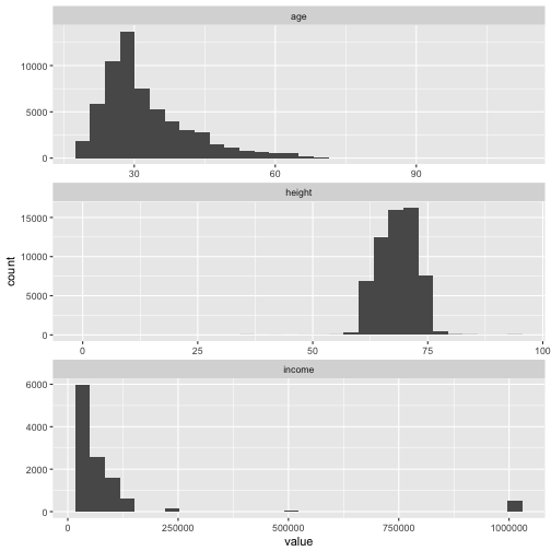
Especially income may be problematic.
Find out more on gather eg., here.
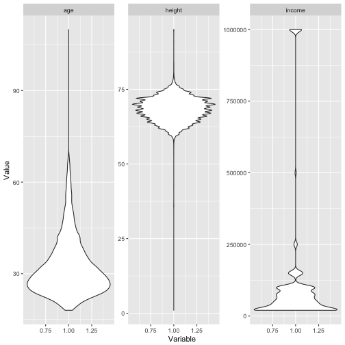
Box plots (or violin plots/bean plots) may also be a way:
data %>%
  select_if(is.numeric) %>%
  gather %>%
  ggplot(aes(x = 1, y = value)) + facet_wrap(~ key, scales = "free") +
  geom_violin() +
  ylab("Value") +
  xlab("Variable")
## Warning: Removed 48445 rows containing non-finite values (stat_ydensity).
Identify variables with unique values
Similar to outliers, for categorical variable we can look whether some values are seldom, e.g, only 0.1% of the times. What “often” or “barely” is, depends on … you!
library(purrr)

data %>%
  select_if(negate(is.numeric)) %>%
  select(-matches("essay")) %>%
  select(-last_online) %>%
  gather %>%
  ggplot(aes(x = value)) + geom_bar() +
  facet_wrap(~ key, scales = "free", ncol = 3)
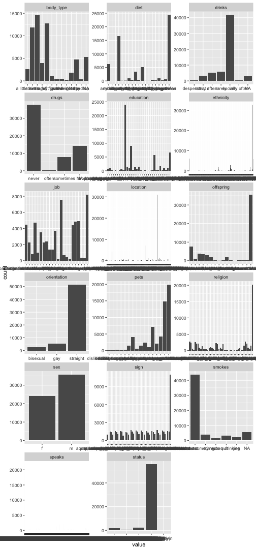
Pooh, that takes ages to plot. And does not look too pretty. Maybe better don’t plot, since we are not after exploration, but just want to know if something is going wrong.
Maybe it is better if we do the following:
for each non-numeric variable do divide most frequent category by least frequent category
This gives an indication whether some categories are quite frequent in relation to others.
data %>%
  select_if(is.character) %>%
  summarise_each(funs(max(table(.)/(min(table(.)))))) %>%
  arrange %>%
  kable
| body_type | diet | drinks | drugs | education | ethnicity | job | location | offspring | orientation | pets | religion | sex | sign | smokes | speaks | status | essay0 |
|---|---|---|---|---|---|---|---|---|---|---|---|---|---|---|---|---|---|
| 74 | 1507.727 | 129.7516 | 92.00976 | 2178.091 | 32831 | 37.20098 | 31064 | 360 | 18.65052 | 336.6818 | 209.5385 | 1.485632 | 43.46341 | 29.65946 | 21828 | 5569.7 | 14 |
Plausibility check
Plausibility check can includes checking orders of magnitude, looking for implausible values (negative body weight), among others. A good starter is to differentiate between numeric and non-numeric variables.
Numeric
data %>%
  select_if(is.numeric) %>%
  map(summary)
## $age
##    Min. 1st Qu.  Median    Mean 3rd Qu.    Max.
##   18.00   26.00   30.00   32.34   37.00  110.00
##
## $height
##    Min. 1st Qu.  Median    Mean 3rd Qu.    Max.    NA's
##     1.0    66.0    68.0    68.3    71.0    95.0       3
##
## $income
##    Min. 1st Qu.  Median    Mean 3rd Qu.    Max.    NA's
##   20000   20000   50000  104400  100000 1000000   48442
The function map comes from package purrr; it maps each selected column to the function summary.
For instance, the max. age of 110 appears somewhat high… And the min. height of 1 should rather be excluded before further operations start. For income similar reasoning applies.
Non-numeric
Let’s do not look at all these essay variables here, because “strange” values are not so straight forward to identify compared to more normal categorical variables (with less distinct values).
data %>%
  select(-matches("essay")) %>%
  select_if(is.character) %>%
  mutate_all(factor) %>%
  map(summary)
Output truncated, TL;DR
We need to convert to factor because for character variables, no nice summary is available of the shelf.
Highly correlated variables
data %>%
  select_if(is.numeric) %>%
  cor
##        age height income
## age      1     NA     NA
## height  NA      1     NA
## income  NA     NA      1
Constants/ near zero variance variables
Applies to numeric variables obviously.
data %>%
  select_if(is.numeric) %>%
  na.omit %>%
  summarise_all(c("sd", "IQR"))
##     age_sd height_sd income_sd age_IQR height_IQR income_IQR
## 1 9.746844  4.003725  201433.5      12          5      80000
Rename many variables
ncol_data <- ncol(data)
names_data_new <- paste("V",1:ncol_data, sep = "")
dummy <- data
names(dummy) <- names_data_new
Recode values
A quite frequent use case is to get “strange” value or variables names in order, e.g., “variable 2” or “I rather not say” (including blanks or some other non-normal stuff).
One approach is to use dplyr::recode.
dplyr::distinct(data, body_type)
##         body_type
## 1  a little extra
## 2         average
## 3            thin
## 4        athletic
## 5             fit
## 6            <NA>
## 7          skinny
## 8           curvy
## 9    full https://sebastiansauer.github.io/images/2017-02-13d
## 10         jacked
## 11 rather not say
## 12        used up
## 13     overweight
dummy <- dplyr::recode(data$body_type, `a little extra` = "1")
unique(dummy)
##  [1] "1"              "average"        "thin"           "athletic"
##  [5] "fit"            NA               "skinny"         "curvy"
##  [9] "full https://sebastiansauer.github.io/images/2017-02-13d"   "jacked"         "rather not say" "used up"
## [13] "overweight"
A second approach is to use base::levels for factors.
dummy <- data$body_type
dummy <- factor(dummy)
levels(dummy)
##  [1] "a little extra" "athletic"       "average"        "curvy"
##  [5] "fit"            "full https://sebastiansauer.github.io/images/2017-02-13d"   "jacked"         "overweight"
##  [9] "rather not say" "skinny"         "thin"           "used up"
levels(dummy) <- 1:12
levels(dummy)
## [1] "1" "2" "3" "4" "5" "6" "7" "8" "9" "10" "11" "12"
I do not use plyr:mapvalues because plyr can interfere with dplyr (and dplyr seems more helpful to me).
Center/ scale variables
As often, several approaches. One is:
data %>%
  select_if(is.numeric) %>%
  scale() %>%
  head
##             age      height     income
## [1,] -1.0938888  1.67836042         NA
## [2,]  0.2813681  0.42673429 -0.1211069
## [3,]  0.5987351 -0.07391616         NA
## [4,] -0.9880998  0.67705952 -0.4189719
## [5,] -0.3533659 -0.57456662         NA
## [6,] -0.3533659 -0.32424139         NA
base::scale performs a z-transformation of the matrix (like object) given as input.
But wait; one issue is that the data frame now consists of the numeric variables only. We have to manually knit it together with the rest of the party. Not so convenient. Rather, try this:
data %>%
  select(-matches("essay")) %>%
  mutate_if(is.numeric, scale) %>%
  glimpse
## Observations: 59,946
## Variables: 21
## $ age         <dbl> -1.09388884, 0.28136809, 0.59873508, -0.98809985, ...
## $ body_type   <chr> "a little extra", "average", "thin", "thin", "athl...
## $ diet        <chr> "strictly anything", "mostly other", "anything", "...
## $ drinks      <chr> "socially", "often", "socially", "socially", "soci...
## $ drugs       <chr> "never", "sometimes", NA, NA, "never", NA, "never"...
## $ education   <chr> "working on college/university", "working on space...
## $ ethnicity   <chr> "asian, white", "white", NA, "white", "asian, blac...
## $ height      <dbl> 1.67836042, 0.42673429, -0.07391616, 0.67705952, -...
## $ income      <dbl> NA, -0.1211069, NA, -0.4189719, NA, NA, NA, NA, NA...
## $ job         <chr> "transportation", "hospitality / travel", NA, "stu...
## $ last_online <dttm> 2012-06-28 20:30:00, 2012-06-29 21:41:00, 2012-06...
## $ location    <chr> "south san francisco, california", "oakland, calif...
## $ offspring   <chr> "doesn't have kids, but might want them", "doesn't...
## $ orientation <chr> "straight", "straight", "straight", "straight", "s...
## $ pets        <chr> "likes dogs and likes cats", "likes dogs and likes...
## $ religion    <chr> "agnosticism and very serious about it", "agnostic...
## $ sex         <chr> "m", "m", "m", "m", "m", "m", "f", "f", "f", "m", ...
## $ sign        <chr> "gemini", "cancer", "pisces but it doesn't matter"...
## $ smokes      <chr> "sometimes", "no", "no", "no", "no", "no", NA, "no...
## $ speaks      <chr> "english", "english (fluently), spanish (poorly), ...
## $ status      <chr> "single", "single", "available", "single", "single...
If we only want to center (or something similar), we could do
data %>%
  mutate_if(is.numeric, funs(. - mean(.))) %>%
  head
##         age      body_type              diet   drinks     drugs
## 1 -10.34029 a little extra strictly anything socially     never
## 2   2.65971        average      mostly other    often sometimes
## 3   5.65971           thin          anything socially      <NA>
## 4  -9.34029           thin        vegetarian socially      <NA>
## 5  -3.34029       athletic              <NA> socially     never
## 6  -3.34029        average   mostly anything socially      <NA>
##                           education           ethnicity height income
## 1     working on college/university        asian, white     NA     NA
## 2             working on space camp               white     NA     NA
## 3    graduated from masters program                <NA>     NA     NA
## 4     working on college/university               white     NA     NA
## 5 graduated from college/university asian, black, other     NA     NA
## 6 graduated from college/university               white     NA     NA
##                              job         last_online
## 1                 transportation 2012-06-28 20:30:00
## 2           hospitality / travel 2012-06-29 21:41:00
## 3                           <NA> 2012-06-27 09:10:00
## 4                        student 2012-06-28 14:22:00
## 5    artistic / musical / writer 2012-06-27 21:26:00
## 6 computer / hardware / software 2012-06-29 19:18:00
##                          location                              offspring
## 1 south san francisco, california doesn't have kids, but might want them
## 2             oakland, california doesn't have kids, but might want them
## 3       san francisco, california                                   <NA>
## 4            berkeley, california                      doesn't want kids
## 5       san francisco, california                                   <NA>
## 6       san francisco, california doesn't have kids, but might want them
##   orientation                      pets
## 1    straight likes dogs and likes cats
## 2    straight likes dogs and likes cats
## 3    straight                  has cats
## 4    straight                likes cats
## 5    straight likes dogs and likes cats
## 6    straight                likes cats
##                                   religion sex
## 1    agnosticism and very serious about it   m
## 2 agnosticism but not too serious about it   m
## 3                                     <NA>   m
## 4                                     <NA>   m
## 5                                     <NA>   m
## 6                                  atheism   m
##                           sign    smokes
## 1                       gemini sometimes
## 2                       cancer        no
## 3 pisces but it doesn't matter        no
## 4                       pisces        no
## 5                     aquarius        no
## 6                       taurus        no
##                                                  speaks    status
## 1                                               english    single
## 2 english (fluently), spanish (poorly), french (poorly)    single
## 3                                  english, french, c++ available
## 4                              english, german (poorly)    single
## 5                                               english    single
## 6                    english (fluently), chinese (okay)    single
##                                                                                                                                         essay0
## 1 about me:    i would love to think that i was some some kind of intellectual: either the dumbest smart guy, or the smartest dumb guy. can't
## 2 i am a chef: this is what that means.  1. i am a workaholic.  2. i love to cook regardless of whether i am at work.  3. i love to drink and
## 3 i'm not ashamed of much, but writing public text on an online dating site makes me pleasantly uncomfortable. i'll try to be as earnest as po
## 4                                                                                                    i work in a library and go to school. . .
## 5 hey how's it going? currently vague on the profile i know, more to come soon. looking to meet new folks outside of my circle of friends. i'm
## 6 i'm an australian living in san francisco, but don't hold that against me. i spend most of my days trying to build cool stuff for my company
That’s it; happy analyzing!