Thanks to my student Marie Halbich who took the pains to collect the data!
At times, your data set will be in “wide” format, i.e, many columns in comparison to rows. For some analyses however, it is more suitable to have the data in “long” format. That is, many rows in comparison to columns.
Let’s have a look at this data set, for example.
d <- read.csv("https://sebastiansauer.github.io/data/facial_beauty_raw.csv")
This is the data from a study tapping into the effect of computerized “beautification” of some faces on subjective “like”.
In short, two strawpersons were present either in “natural form” or “beautified” with some computer help. Note that the design is a between-group design with the factor “strawpersons” (A and B) and the factor “presentation” (natural vs. beautified).
library(dplyr)
glimpse(d)
#> Observations: 1,440
#> Variables: 23
#> $ X                                          <int> 1, 2, 3, 4, 5, 6, 7...
#> $ Item                                       <int> 1, 2, 3, 4, 5, 6, 7...
#> $ Alter                                      <int> 26, 31, 35, 34, 31,...
#> $ girl_C_unbearbeitet_Likes                  <int> NA, 1, 1, 1, 1, 1, ...
#> $ girl_C_unbearbeitet_Dislikes               <int> 1, NA, NA, NA, NA, ...
#> $ girl_C_unbearbeitet_Superlikes             <int> NA, NA, NA, NA, NA,...
#> $ girl_C_unbearbeitet_Kontaktaufnahmen       <int> NA, 1, 1, NA, 1, 1,...
#> $ girl_C_unbearbeitet_keine_Kontaktaufnahmen <int> 1, NA, NA, 1, NA, N...
#> $ girl_C_bearbeitet_Like                     <int> NA, NA, NA, NA, NA,...
#> $ girl_C_bearbeitet_Dislike                  <int> NA, NA, NA, NA, NA,...
#> $ girl_C_bearbeitet_Superlike                <int> NA, NA, NA, NA, NA,...
#> $ girl_C_bearbeitet_Kontaktaufnahme          <int> NA, NA, NA, NA, NA,...
#> $ girl_C_bearbeitet_keine_Kontaktaufnahme    <int> NA, NA, NA, NA, NA,...
#> $ girl_A_unbearbeitet_Like                   <int> NA, NA, NA, NA, NA,...
#> $ girl_A_unbearbeitet_Dislike                <int> NA, NA, NA, NA, NA,...
#> $ girl_A_unbearbeitet_Superlike              <int> NA, NA, NA, NA, NA,...
#> $ girl_A_unbearbeitet_Kontaktaufnahme        <int> NA, NA, NA, NA, NA,...
#> $ girl_A_unbearbeitet_keine_Kontaktaufnahme  <int> NA, NA, NA, NA, NA,...
#> $ girl_A_bearbeitet_Like                     <int> NA, NA, NA, NA, NA,...
#> $ girl_A_bearbeitet_Dislike                  <int> NA, NA, NA, NA, NA,...
#> $ girl_A_bearbeitet_Superlike                <int> NA, NA, NA, NA, NA,...
#> $ girl_A_bearbeitet_Kontaktaufnahme          <int> NA, NA, NA, NA, NA,...
#> $ girl_A_bearbeitet_keine_Kontaktaufnahme    <int> NA, NA, NA, NA, NA,...
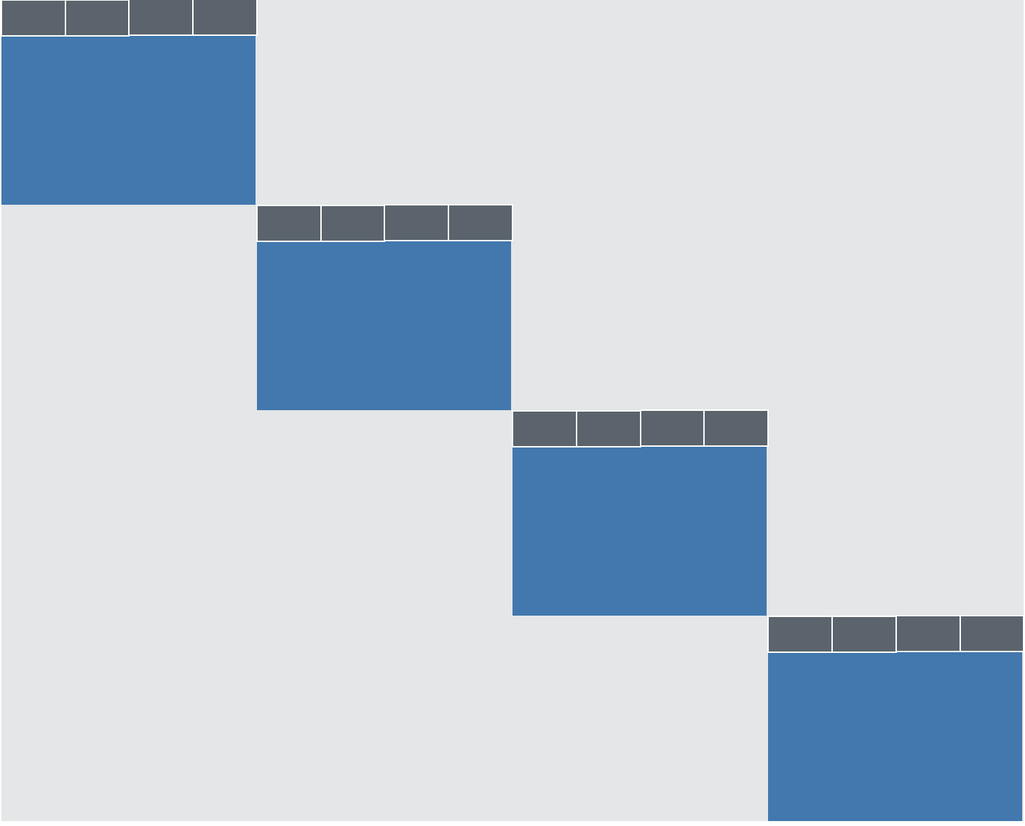
On closer inspection, we recognize a great number of missing values. In fact, the data frame is structured like this:
library(knitr)
include_graphics("facial_beauty.png")

Where each blue rectangle represents the “core” data set for one of the four conditions (mentioned above). All the grey area represents vast deserts of NAs.
That said, the data set would be much nicer if the four “core data sets” would be aligned beneath each other like this:
library(knitr)
include_graphics("beauty_aligned.png")

Of course, this would demand that the columns be the same in each blue square. And we will need a column indicating the value of the factor “strawperson” and a columnd for “presentation”. We don’t need column headers for times, only once, as shown on the diagram.
Cutting out the sub data frames
So we will “cut out” each sub data frame (blue rectangle) and stick them together one beneath another.
Let’s start for “girl C” and “unbearbeitet” (meaning “raw” or “natural”).
d_C_raw <-
  d %>%
  dplyr::select(dplyr::contains("girl_C_unbearbeitet"), Alter)
The helper function contains is handy to choose the right columns.
Now we get rid of the empty lines. We exclude all rows where only NAs appear (not looking at Alter, were no NAs will pop up).
d_C_raw <-
  d_C_raw %>%
    filter(!is.na(girl_C_unbearbeitet_Likes) |
          !is.na(girl_C_unbearbeitet_Dislikes) |
          !is.na(girl_C_unbearbeitet_Superlikes)|
            !is.na(girl_C_unbearbeitet_Kontaktaufnahmen) |
            !is.na(girl_C_unbearbeitet_keine_Kontaktaufnahmen))
Note that the | operator means OR (logical OR). So we way that we want any raw where there is no NA at girl_C_unbearbeitet_Likes or no NA at girl_C_unbearbeitet_Dislikes or no NA at girl_C_unbearbeitet_Superlikes.
Now we have our first “data cubicle”. Let’s repeat that for the other 3 data cubicles.
Data frame for girl C “beautified”:
d_C_beauty <-
  d %>%
  dplyr::select(dplyr::contains("girl_C_bearbeitet"), Alter)

d_C_beauty <-
 d_C_beauty %>%
    filter(!is.na(girl_C_bearbeitet_Like) |
          !is.na(girl_C_bearbeitet_Dislike) |
          !is.na(girl_C_bearbeitet_Superlike) |
            !is.na(girl_C_bearbeitet_Kontaktaufnahme) |
            !is.na(girl_C_bearbeitet_keine_Kontaktaufnahme))
The variable names are probably somewhat verbose, but let’s not discuss that here. Also note that the names are not fully consistent; at times they come in plural and at times in singular form.
Now girl A, natural:
d_A_raw <-
  d %>%
  dplyr::select(dplyr::contains("girl_A_unbearbeitet"), Alter)

d_A_raw <-
 d_A_raw %>%
    filter(!is.na(girl_A_unbearbeitet_Like) |
          !is.na(girl_A_unbearbeitet_Dislike) |
          !is.na(girl_A_unbearbeitet_Superlike) |
            !is.na(girl_A_unbearbeitet_Kontaktaufnahme) |
            !is.na(girl_A_unbearbeitet_keine_Kontaktaufnahme))
Once more for girl A, processed:
d_A_beauty <-
  d %>%
  dplyr::select(dplyr::contains("girl_A_bearbeitet"), Alter)

d_A_beauty <-
 d_A_beauty %>%
    filter(!is.na(girl_A_bearbeitet_Like) |
          !is.na(girl_A_bearbeitet_Dislike) |
          !is.na(girl_A_bearbeitet_Superlike) |
            !is.na(girl_A_bearbeitet_Kontaktaufnahme) |
            !is.na(girl_A_bearbeitet_keine_Kontaktaufnahme))
Adjust names of sub data frames
Before we can bind the sub data frames together, we have to make sure the names of the columns are identical. So let’s do that now. In addition, we need to save the information about the study factors (natural vs. processed; girl A vs. girl C).
d_A_beauty$girl <- "A"
d_A_beauty$presentation <- "beauty"
d_A_raw$girl <- "A"
d_A_raw$presentation <- "natural"


d_C_beauty$girl <- "C"
d_C_beauty$presentation <- "beauty"
d_C_raw$girl <- "C"
d_C_raw$presentation <- "natural"
OK, now the names of the variables:
names_cols <- c("like_yes", "like_no", "superlike_yes", "contact_yes", "contact_no", "age", "girl", "presentation")

names(d_A_raw) <- names_cols
names(d_A_beauty) <- names_cols
names(d_C_raw) <- names_cols
names(d_C_beauty) <- names_cols
Bind sub data frames
Now we are ready to bind the four sub data frames into one, by placing the four pieces underneath each other:
d_long <- bind_rows(d_A_raw, d_A_beauty, d_C_raw, d_C_beauty)
Wow! Now we have reformated our data frame from “wide” format to “long” format. Long ride.
Unite columns
Note that some columns are dependent: a 1 in like corresponds to NA in dislike and a NA in superlike. We can merge these columns into one. Same story for contact.
First, recode NAs to 0 as this it what they mean here.
d_long <-
  d_long %>%
  mutate_at(vars(like_yes, like_no, superlike_yes, contact_yes, contact_no),
            recode, .missing = 0, `1` = 1)
A quick check:
count(d_long, like_yes)
#> # A tibble: 2 × 2
#>   like_yes     n
#>      <dbl> <int>
#> 1        0   404
#> 2        1  1036
count(d_long,like_no)
#> # A tibble: 2 × 2
#>   like_no     n
#>     <dbl> <int>
#> 1       0  1036
#> 2       1   404
Seems OK.
Next, merge the three “like columns” into one using dplyr::case_when:
d_long <-
  d_long %>%
  mutate(like = case_when(
    d_long$like_yes == 1 ~ "like",
    d_long$like_no == 1 ~ "dislike",
    d_long$superlike_yes == 1 ~ "superlike"))
Note that case_when will fail if there are NAs in your vector (without an helpful error).
Now we can drop the initial three “like columns”.
d_long <-
  d_long %>%
  select(-c(like_yes, like_no, superlike_yes))
And now same story for the two “contact columns”.
Wait, if 1 in contact_yes means 0 in contact_no, then we are already done.
Let’s look at the counts of the two variables:
count(d_long, contact_yes)
#> # A tibble: 2 × 2
#>   contact_yes     n
#>         <dbl> <int>
#> 1           0   853
#> 2           1   587
count(d_long, contact_no)
#> # A tibble: 2 × 2
#>   contact_no     n
#>        <dbl> <int>
#> 1          0   585
#> 2          1   855
Hm, that’s no exact match, but nearly. Probably some typing errors or something similar. So we can just rename one variable, drop the other, and that’s it.
d_long <-
  d_long %>%
  rename(contact = contact_yes) %>%
  select(-contact_no)
Debrief
That’s about it. We have now a data frame in “long” format. This version is more adequat for many analyses. Have fun!
Session info
sessionInfo()
#> R version 3.3.2 (2016-10-31)
#> Platform: x86_64-apple-darwin13.4.0 (64-bit)
#> Running under: macOS Sierra 10.12.2
#>
#> locale:
#> [1] en_US.UTF-8/en_US.UTF-8/en_US.UTF-8/C/en_US.UTF-8/en_US.UTF-8
#>
#> attached base packages:
#> [1] stats     graphics  grDevices utils     datasets  methods   base
#>
#> other attached packages:
#> [1] knitr_1.15.1 dplyr_0.5.0
#>
#> loaded via a namespace (and not attached):
#>  [1] Rcpp_0.12.8         codetools_0.2-15    digest_0.6.11
#>  [4] rprojroot_1.1       assertthat_0.1      R6_2.2.0
#>  [7] DBI_0.5-1           backports_1.0.4     magrittr_1.5
#> [10] evaluate_0.10       highr_0.6           stringi_1.1.2
#> [13] lazyeval_0.2.0.9000 rmarkdown_1.3       tools_3.3.2
#> [16] stringr_1.1.0       rsconnect_0.7       yaml_2.1.14
#> [19] htmltools_0.3.5     tibble_1.2