The variance of some data can be defined in rough terms as the mean of the squared deviations from the mean.

Let’s repeat that because it is important:

Variance: Mean of squared deviations from the mean.

An example helps to illustrate. Assume some class of students are forced to write an exam in a statistics class (OMG). Let’s say the grades range fom 1 to 6, 1 being the best and 6 the worst. We can compute the mean of this class (eg., 2.3); once we know the mean, we can subtract the mean from each individual grade. If Anna scored a 3 (OK but not exciting), “her” residual, delta or deviation would 3 - 2.3 = 0.7, and so on. The following picture illustrates this example.

library(tidyverse)

# df with students' grades (12 students)
grades_df <- data_frame(grades = c(3,2,4,1,1,2,5,1,1,3,2,2))


# compute deltas (deviations from mean)
grades_df %>% 
  mutate(grades_Delta = grades - mean(grades),
         Student = factor(row_number())) -> grades_df 

# now plot 
grades_df%>% 
  ggplot(aes(x = Student, y = grades)) + geom_point() +
  geom_hline(yintercept = mean(grades_df$grades), color = "firebrick") +
  geom_linerange(aes(x = Student, ymin = grades, ymax = grades - grades_Delta), color = "blue") 

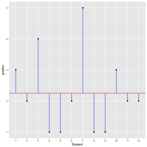
The vertical blue lines look a bit like little sticks…

In this example, the vertical blue sticks indicate the individual delta. Now try to envision the “average” length of the stick. That’s something similar to the variance but not exactly the same. We have to to square each stick, and then only take the avarage.

In R, a fancy (piped) way to compute the variance is this:

grades_df$grades %>% 
  `-`(mean(grades_df$grades)) %>% 
  `^`(2) %>% 
  mean

## [1] 1.520833

Literally, in plain English, this code means:

Take the data frame “grades_df”, and from there the column “grades”. Then
subtract the mean of this column. Then
take it to the 2nd power (square it, that is). Then
compute the mean of the numbers.

More formally, the variance of some empirical data is defined as

$$ s^2 = \frac{1}{n}\sum{(x-\bar{x})^2} $$.

And for infinite variables (whatever that is) it is defined as:

$$ s^2 = \varnothing \lbrack (x - \varnothing{x})^2 \rbrack $$.

Note that $$\varnothing$$ means “the mean on the long run” (infinitely long, to be sure).

Which is exactly the same as the R code above; slightly more complicated, I feel, because the steps are nested (because of the brackets). In the R code above, we “sequentialized” the steps, which renders the thing more tangible.

Note that the R function var does not divide by n but by n-1. However, for larger samples, the error is negligible. The reason is that R computes the so-called “sample variance”, that is the estimate of the population variance based on the sample data. Thus, depending on whether you are interested in a guess of the population variance or just the variance of your data at hand, the one or the other is (slightly) more appopriate. If you were to know to population variance, then again you’d divide by n(not by n-1). Here, we just divide by n and by happy.

In general, my opinion is not to worry too much about tiny details (for the purpose given), but rather to try to grasp the big pictures. So we won’t elaborate here on that further.

Note that the dice throws are independent with each others, they are not correlated.

Simulate dice throwing

With this understanding of the variance in mind, let’s continue. Let’s make R throw some dice to illustrate the additivity property of the variance.

Hey R: throw a normal die reps = 1e05 times and plot the results:

reps <- 1e05
dice <- sample(x = c(1:6), size = reps, replace = TRUE)
dice <- tibble(dice)

ggplot(dice) +
  aes(x = dice) +
  geom_histogram()

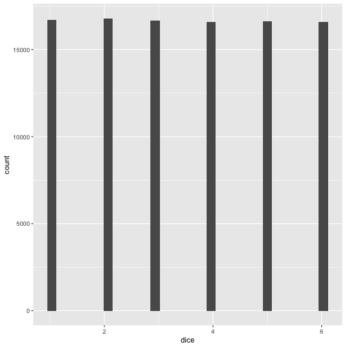
OK, fair enough; each side appeared more or less equally often.

Now, what' the mean and the variance?

var(dice$dice)

## [1] 2.915413

mean(dice$dice)

## [1] 3.494

OK, plausible.

Now, we are concerned with the additivity of the variance. So we are supposed to some stuff up! Suppose we repeat our dice throwing experiment, but now with 2 dices (instead of 1). After each throw, we sum up the score. After some hard thinking we feel reassured that this should yield a number between 2 and 12. Let’s have a look at the plot, as we want to get an intuitive understanding.

dice1 <- sample(x = c(1:6), size = reps, replace = TRUE)

dice2 <- sample(x = c(1:6), size = reps, replace = TRUE)

dice_sum <- dice1 + dice2
# dice_sum <- sum(dice1, dice2) this will not work!

dice_sum <- tibble(dice_sum)

ggplot(dice_sum) +
  aes(x = dice_sum) +
  geom_histogram() +
  scale_x_continuous(breaks = 1:12)  

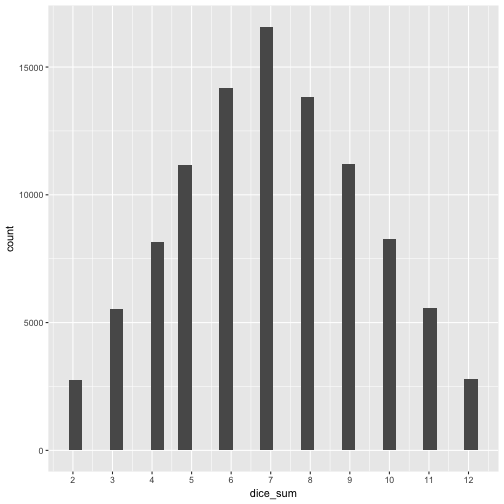
But what about mean and variance? Let’s see.

mean(dice_sum$dice_sum)

## [1] 7.00482

var(dice_sum$dice_sum)

## [1] 5.808515

It appears that the means are adding up, which makes sense, if you think about it. Same for the variance, it adds up!

Sum up k variables

As a last step, let’s add up, say, $$k = 10$$ variables (die throws) to further strengthen our argument.

First, we make up some data with k columns of dice throws.

d <- list()
k <- 10 
for (i in 1:k){
  d[i] <- list(sample(x = c(1:6), size = reps, replace = TRUE))
}

d <- rbind.data.frame(d)
names(d) <- paste("V",1:k, sep = "")

Now sum up the score of each of the throws with k dice.

d$sum_throw <- rowSums(d[, 1:10])

We expect the variance to be about k times var(one_die_throw).

var(d$sum_throw)

## [1] 29.29128

Which is what we find. Similarly for the mean:

mean(d$sum_throw)

## [1] 34.99714

OK.

What about sd?

Does this property hold with the sd as well?

So, what’s the sd in each of the die throws?

sds <- apply(d[, 1:10], 2, sd)
sds

##       V1       V2       V3       V4       V5       V6       V7       V8 
## 1.707311 1.704684 1.707218 1.705219 1.706854 1.709697 1.709320 1.703763 
##       V9      V10 
## 1.704847 1.710907

And their sum is then 17.0698202.

But what is the sd of the sum score of the k=10 throws?

sd(d$sum_throw)

## [1] 5.412142

These two numbers are obviously not equal. So the additivity property does not hold for the sd.

More formally

Thus, we can state with some confidence:

$$Var(A+B+C+ …) = Var(A) + Var(B) + Var(C) + …$$,

where Var means variance and A, B, C, … are some variables such as dice throws.

Subtracting two variables

OK, we have seen that the variance is additive in the sense that if we sum up som arbitrary number of variables, the variance of the sum score equals the sum of the individual variances (approximately, not exactly).

But what about subtracting two variables. Does the variance get smaller in the same way, too? Let’s try and see.

dice1 <- sample(x = c(1:6), size = reps, replace = TRUE)

dice2 <- sample(x = c(1:6), size = reps, replace = TRUE)

dice_diff <- dice1 - dice2

dice_diff <- tibble(dice_diff)

ggplot(dice_diff) +
  aes(x = dice_diff) +
  geom_histogram() +
  scale_x_continuous(breaks = -5:5)  

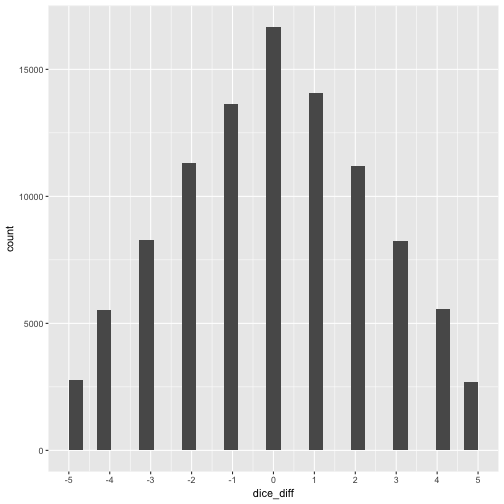
Obviously, if we subtract one die score from the other the result must come down between -5 and +5. But what about mean and variance? Let’s see.

mean(dice_diff$dice_diff)

## [1] -0.00232

var(dice_diff$dice_diff)

## [1] 5.813533

Interesting. The mean does what it should, it balances out again. But what about the variance? It again adds up! We see that the range is 11. Compare the “width” (range) of the individual dice throws:

ggplot(tibble(dice1)) +
  aes(x = dice1) +
  geom_histogram() +
  scale_x_continuous(breaks = 1:6)  

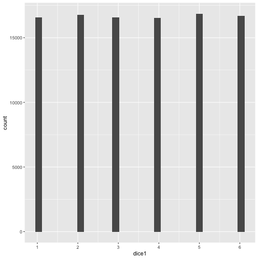
The range is smaller, ie. 6. So, again, it appears that despite us subtracting variables, the variance keeps adding up!.

Formal stuff

Note that in general, the variance of some (infinite) distribution is defined as follows:

$$Var(X) = \varnothing \lbrack (X - \varnothing X ) ^2 \rbrack $$ Here $$\varnothing$$ means “long term average” or “expected value”. X is just some variable such as a fair die throw.

This formula can be rearranged to

$$Var(X) = \varnothing(X^2) - (\varnothing X)^2$$

Mnemonic is “mean of square minus square of mean”; see here for details.

Similarly, for the sum of two variables, X and Y, we substitute X by X+Y:

$$Var(X+Y) = \varnothing \lbrack(X+Y) \rbrack ^2 - \lbrack \varnothing(X+Y) \rbrack^2 =$$

Let’s open the first bracket (first binomic formula):

$$ \varnothing \lbrack (X^2 + 2XY + Y^2 \rbrack - (\varnothing X + \varnothing Y) ^2 =$$

Now pull the “mean symbol” to each part of the expression:

$$ \varnothing X^2 + 2\varnothing(XY) + \varnothing(Y^2) - \lbrack(\varnothing X)^2 + 2 \varnothing X \varnothing Y + (\varnothing Y)^2 ) $$

Get rid of some brackets:

$$ \varnothing X^2 + 2\varnothing(XY) + \varnothing(Y^2) - (\varnothing X)^2 - 2 \varnothing X \varnothing Y - (\varnothing Y)^2 = $$

And we recognize some known expressions:

$$ \underbrace{\varnothing X^2 - (\varnothing X)^2}{\substack{Var(X)}} + 2\underbrace{(\varnothing XY - \varnothing X \varnothing Y)}{\substack{Cov(X,Y)}} + \underbrace{\varnothing (Y^2) - (\varnothing Y)^2}_{\substack{Var(Y)}}$$

If X and Y are independent (uncorrelated) then Cov(X,Y) = 0. So we end up with:

$$Var(X+Y) = Var(X) + Var(Y)$$

Debrief

Well, we have dived in to the fact that the variance is additive. That is the variance of a sum (or difference) of k variables equals the sum of the variance of each variance (see expression above).

To come to this result we have used some simulation which has the advantage that it is less abstract. Then we flipped to some more rigorous proof (but which is less tangible).

What do we need all that stuff for? Basically a number of of statistical tests or procedures use this property such as the ANOVA or R squared. Maybe equally of more important, we here have an answer why the variance is used for descriptive statistics where some other measure appears more tangible. As the variance has this nice feature which we can use for later steps in data analytic projects, we compute it right at the beginning.