We are often interested in the question whether two variables are “associated”, “correlated” (I mean the normal English term) or “dependent”. What exactly, or rather in normal words, does that mean? Let’s look at some easy case.
NOTE: The example has been updated to reflect a more tangible and sensible scenario (find the old one in the previous commit at Github).
Titanic data
For example, let’s look at survival rates of the Titanic disaster, to see whether the probability of survival (event A) depends on the whether you embarked for 1st class (event B).
Let’s load the data and have a look at them.
data(titanic_train, package = "titanic")

library(tidyverse)  # plotting and data mungling
library(pander)  # for markdown tables

data <- titanic_train
glimpse(data)
## Observations: 891
## Variables: 12
## $ PassengerId <int> 1, 2, 3, 4, 5, 6, 7, 8, 9, 10, 11, 12, 13, 14, 15,...
## $ Survived    <int> 0, 1, 1, 1, 0, 0, 0, 0, 1, 1, 1, 1, 0, 0, 0, 1, 0,...
## $ Pclass      <int> 3, 1, 3, 1, 3, 3, 1, 3, 3, 2, 3, 1, 3, 3, 3, 2, 3,...
## $ Name        <chr> "Braund, Mr. Owen Harris", "Cumings, Mrs. John Bra...
## $ Sex         <chr> "male", "female", "female", "female", "male", "mal...
## $ Age         <dbl> 22, 38, 26, 35, 35, NA, 54, 2, 27, 14, 4, 58, 20, ...
## $ SibSp       <int> 1, 1, 0, 1, 0, 0, 0, 3, 0, 1, 1, 0, 0, 1, 0, 0, 4,...
## $ Parch       <int> 0, 0, 0, 0, 0, 0, 0, 1, 2, 0, 1, 0, 0, 5, 0, 0, 1,...
## $ Ticket      <chr> "A/5 21171", "PC 17599", "STON/O2. 3101282", "1138...
## $ Fare        <dbl> 7.2500, 71.2833, 7.9250, 53.1000, 8.0500, 8.4583, ...
## $ Cabin       <chr> "", "C85", "", "C123", "", "", "E46", "", "", "", ...
## $ Embarked    <chr> "S", "C", "S", "S", "S", "Q", "S", "S", "S", "C", ...
Look at the package description for some details on the variables.
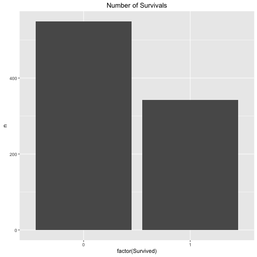
Let’s look at the survival rate in general, that is to say to probability of A - irrespective of the the class (1st class or not 1st class).
data %>%
  count(Survived) %>%
  ggplot +
  aes(x = factor(Survived), y = n) +
  geom_bar(stat = "identity") +
  ggtitle("Number of Survivals") +
  theme(plot.title = element_text(hjust = .5))
Maybe that’s a better plot:
data %>%
  count(Survived) %>%
  ggplot +
  aes(x = factor(1), fill = factor(Survived), y = n) +
  geom_bar(stat = "identity") +
  ggtitle("Number of Survivals") +
  theme(plot.title = element_text(hjust = .5)) +
  xlab("")
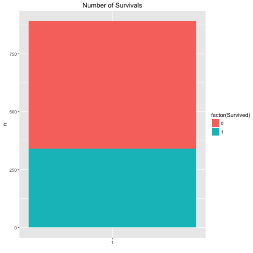
The exact figures are for the survivals are:
data %>%
  count(Survived)
## # A tibble: 2 × 2
##   Survived     n
##      <int> <int>
## 1        0   549
## 2        1   342
The exact figures are for the classes (1st vs. other) are:
data %>%
  mutate(Pclass_bin = ifelse(Pclass == 1, "1st", "not_1st")) %>%
  count(Pclass_bin)
## # A tibble: 2 × 2
##   Pclass_bin     n
##        <chr> <int>
## 1        1st   216
## 2    not_1st   675
… and the number of passengers per class (1st class vs. other classes) is:
data %>%
  mutate(Pclass_bin = ifelse(Pclass == 1, "1st", "not_1st")) %>%
  count(Survived, Pclass_bin)
## Source: local data frame [4 x 3]
## Groups: Survived [?]
##
##   Survived Pclass_bin     n
##      <int>      <chr> <int>
## 1        0        1st    80
## 2        0    not_1st   469
## 3        1        1st   136
## 4        1    not_1st   206
So, that was warming up. Let’s see what the probability (percentage) of survival is for both 1st class and non-first class.
data %>%
  mutate(Pclass_bin = ifelse(Pclass == 1, "1st", "not_1st")) %>%
  count(Pclass_bin, Survived) %>%
  ggplot +
  aes(x = factor(Pclass_bin), fill = factor(Survived), y = n, labels = n) +
  geom_bar(stat = "identity") +
  ggtitle("Probability of Survivals given Passenager class") +
  theme(plot.title = element_text(hjust = .5))
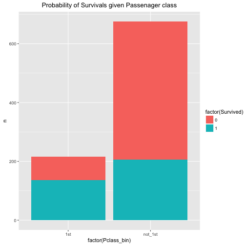
We easily conclude that the probability of survival is associated with passenger class. The probability of survival (event A) given 1st class (event B) is considerably higher than the probability of A given non-B (event B is “not 1st class”).
The exact numbers are:
data %>%
  mutate(Pclass_bin = ifelse(Pclass == 1, "1st", "not_1st")) %>%
  count(Pclass_bin, Survived) -> data_2

data_2
## Source: local data frame [4 x 3]
## Groups: Pclass_bin [?]
##
##   Pclass_bin Survived     n
##        <chr>    <int> <int>
## 1        1st        0    80
## 2        1st        1   136
## 3    not_1st        0   469
## 4    not_1st        1   206
pandoc.table(data_2, style = "rmarkdown")
| Pclass_bin | Survived | n |
|---|---|---|
| 1st | 0 | 80 |
| 1st | 1 | 136 |
| not_1st | 0 | 469 |
| not_1st | 1 | 206 |
General notion of stochastic independence
A typical definition of stochastic (or statistic) independence is this:
That means in plain English, that the probability of A (survival) given B (1st class) is equal to A irrespective of B, that means irrespective of B is the case or non-B is the case. In short, that would mean the survival probability is equal in both cases (B or non-B).
In math-speak:
Here, the “cup” means “OR”.
It than follows that if we deduce
Or more verbose in our Titanic example:
.
In words, whether someone survives is independent from the question of his or her passenger class: Survival probability is the the same in 1st class and in the other classes (“non 1st class”).
Let’s look at the data of our example:
$$p(A) = 342 / (549+342) = 0.38 \
p(nonA) = 549 / (549+342) = 0.62 \
p(B) = 216 / (216 + 675) = 0.24 \
p(nonB) = 675 / (216 + 675) = 0.76 \
p(A|B) = 136 / (80+136) = 0.63 \
p(nonA|B) = 80 / (80+136) = 0.37 \
p(A|nonB) = 206 / (206+469) = 0.31 \
p(nonA|nonB) = 469 / (206+469) = 0.69$$
In R:
p_A <- 342 / (549+342)
p_nonA <- 549 / (549+342)

p_B <- 216 / (216 + 675)
p_nonB <- 549 / (549+342)


p_B <- 216 / (216 + 675)
p_nonB <- 675 / (216 + 675)
p_A_given_B <- 136 / (80+136)
P_nonA_given_B <- 80 / (80+136)

p_A_given_nonB <- 206 / (206+469)
p_nonA_given_nonB <- 469 / (206+469)


p_diff <- p_A_given_B - p_A_given_nonB
p_diff
## [1] 0.3244444
The difference p(A|B) - p(A|nonB) is not zero. Actually it is quite far away: If you are in 1st, your survival rate is 32% higher if you were not in 1st class. Quite strong. However, note that this last step is subjective, no job for statistics.
Finally, let’s look for two variable which are not associated. For example: Shoe size (of adults) and their bank account number.
In our dataset, what about port of Embarkement: Southampton vs. not Southampton and Survival rate.
data %>%
  mutate(Embarked_bin = ifelse(Embarked == "S", "S", "not_S")) %>%
  select(Embarked_bin, Survived) %>%
  count(Embarked_bin, Survived) %>%
  ggplot +
  aes(x = Embarked_bin, y = n, fill = factor(Survived)) +
  geom_bar(stat = "identity")
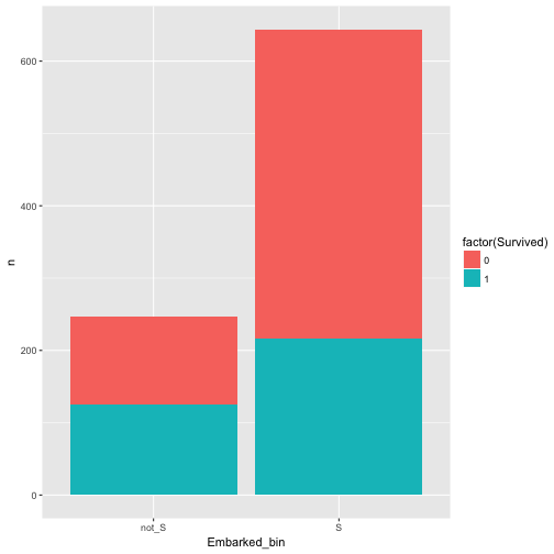
Hm, appears to be related/associated/dependent/correlated.
Maybe better plot like this:
data %>%
  mutate(Embarked_bin = ifelse(Embarked == "S", "S", "not_S")) %>%
  select(Embarked_bin, Survived) %>%
  count(Embarked_bin, Survived) %>%
  ggplot +
  aes(x = Embarked_bin, y = n, fill = factor(Survived)) +
  geom_bar(stat = "identity", position = "fill")
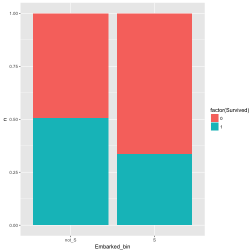
Ah, yes, there is some dependence.
Ok, last try, this is should be a save win: Whether fare is an odd number (eg., 7 Pound) and survival are related.
data %>%
  mutate(Fare_odd = ifelse(round(Fare) %% 2 == 0, "even", "odd")) %>%
  select(Fare_odd, Survived) %>%
  count(Fare_odd, Survived) %>%
  ggplot +
  aes(x = Fare_odd, y = n, fill = factor(Survived)) +
  geom_bar(stat = "identity", position = "fill")
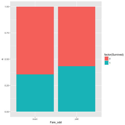
Well, nearly equal, approximately independent, or independent enough for me (as said, that’s subjective).
Concluding remarks
Of course there are numerous ways to “measure” the strength of assocation. Odds ratios, for example, a popular choice. The reason why I like or presented this version is that I find it intuitively appealing. In my teaching I found that the Odds Ratio was somewhat more difficult to grasp at first.
Also note that we where looking at discrete events, not continuous.