Likert scales are psychologists' bread-and-butter tool. Literally, thousands (!) of such “scales” (as they are called, rightfully or not) do exist. To get a feeling: The APA links to this database where 25,000 tests are listed (as stated by the website)! That is indeed an enormous number.
Most of these psychological tests use so called Likert scales (see this Wikipedia article). For example:

(Source: Wikipedia by Nicholas Smith)
Given their widespread use, the question how useful such tests are has arisen many times; see here, here, or here.
For example, Carifio and Perla 2007 assume that underlying each response format ranging from e.g, “agree” to “disagree” there must be an metric attribute. Thus, they hold the philosophical view that each (psychological) attribute must be metric. They do not present any grounds for that stark claim. Similarly, they assume that each of such scales maps an empirical quantitative attribute. And they assume without any consideration that some given items (they call it a scale), automatically measure the same underlying quantity (if existing). Besides their stark language, I am strongly disagree with many points they are rising. Sadly, they fail to mention even the most basic aspects of measurement theory (see here for a nice introduction; read the work of Michell for a more in-depth reasoning).
For example, one proponent that Likert scales generally do exhibit interval (metric) level is is Labovitz, eg., in his 1970 paper, paywalled.
However, other scholars have insisted that Likert scales do not (generally) possess metric level, and that demonstrating metric niveau is quite a delicate job. Maybe the most pronounced critic is Joel Michell, see e.g. this paper.
As a matter of fact, measurement theory is not so easy, if measured by the sheer weight of “foundational” text books, most notably the three volumes by Krantz et al. .
Krantz, D. H., Luce, R. D., Suppes, P., and Tversky, A. (1971), Foundations of measurement, Vol. I: Additive and polynomial representations, New York: Academic Press.
Suppes, P., Krantz, D. H., Luce, R. D., and Tversky, A. (1989), Foundations of measurement, Vol. II: Geometrical, threshold, and probabilistic respresentations, New York: Academic Press.
Luce, R. D., Krantz, D. H., Suppes, P., and Tversky, A. (1990), Foundations of measurement, Vol. III: Representation, axiomatization, and invariance, New York: Academic Press.
Reporting the basics of measurement theory is beyond the scope of this post, but let’s briefly mention that, at least, if one variable is to be taken quantitative (here the same as metric), then it should
- be ordinal
- the distance between adjacent values should be equal (equidistance).
The latter property can be called “additivity”, or at least defines some necessary parts of additivity. (Let’s take ordering (ordinal level) for granted here.)
Equidistance
What is meant by equidistance? It means that, for example, the difference in weight between 1 kg and 2 kg should be equal to the difference in weight between 2 kg and 2 kg. If so (and for many other values 3, 4, 5, … kg as well), we are inclined to say that this variable “kg” exhibits equidistance.
Note that we are not interested in “weight” per se, but in “kg”, or, more precisely, in our measurement device (maybe some old-day balance apparatus) and its claims about weight in kg.
That quite directly yields to a problem of Likert scales: Is the difference between “do not agree at all” and “rather not agree” the same as between “rather not agree” and “strongly agree”?
A similar discussion has been around for school grades.
I think, the short answer is: We cannot take it for granted that the distances are equal; why should they? If we are ignorant or neutral, it appears for more likely that the distances are not equal, as it appears more likely that any two number are different rather than equal.
Sprinters' example
Let’s look at a practical example. Suppose 10 sprinters are running the 100 meters, with different times:
sprinters <- data.frame(
  ranking = 1:10,
  time = c(9.8, 10, 10.6, 13.1, 17.2, 17.3, 17.8, 23, 66, 91.1)
)
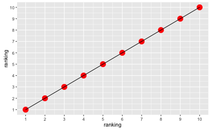
Of course, the rankings appear equidistant:
library(ggplot2)
ggplot(sprinters, aes(x = ranking, y = ranking)) + geom_point(color = "red", size = 5) +
  geom_line() + scale_x_continuous(breaks = 1:10) +
  scale_y_continuous(breaks = 1:10)

But the running times clearly are not:
ggplot(sprinters, aes(x = ranking, y = time)) + geom_point(color = "red", size = 5) +
  geom_line() +
  scale_x_continuous(breaks = 1:10)

Enough values = metric level?
Some say (sorry, did not find a citation, but one of my teachers said so!) that if there are “enough” values, the variable becomes “automagically” metric. I cannot see why this must necessarily happen. Suppose we would not have 10 but 100 sprinters; the picture and the argument would in essence remain the same. Equidistance will not necessarily pop out. It may by chance occur, but it is not a necessity (by far not).
Now, if we were to have many items, can we then infer that equidistance will necessarily come out? Let’s put it this way in our sprinter example: Suppose we had not watched one race, but many (say, 8). Assume that the measurement error is negligible (to make things easier but without loss of generality). If measurement error is negligible, then the actual performance, ie., the sprint times, can be taken to be the “real” (“latent”) sprinting time of the person. Measurement error is not only confined to e.g., imprecision when taking the time, but includes local particularities as wind speed, mood disturbances, bad hair days, etc.
Then, again, I think, the argument remains the same: We would have more data, but in this toy example, the average time values of the sprinters would remain the same as in the example above. So the implications also remain the same. Equidistance is no free lunch.
If ordinal and metric association measures are similar, then what the fuss?
Some argue in this way: Association measures (such as Kendall’s tau) and metric association measures (such as Pearson' r) are often similar.
Hence, it is inferred that it does not matter much if we take the ranks as metric variables. I disagree with that argument.
What follows is inspired by Gigerenzer’s 1981 book (available in German only). Let’s first come up with some data (taken from Gigerenzer’s book, p. 303):
df <- data.frame(
  x = c(-2, -2, -1, 0, 0, 1, 1, 3, 5, 5),
  y = c(0, 0.5, 1, 1.5, 2, 13, 13.5, 14, 14.5, 15),
  ID = 1:10
)
This yields a correlation (Pearson) of
r_pearson <- round(cor(df$x, df$y), 3)
r_pearson
## [1] 0.868
a Spearman correlation of
r_spearman <- round(cor(df$x, df$y, method = "spearman"), 3)
r_spearman
## [1] 0.988
and Kendall’s tau of
tau <- round(cor(df$x, df$y, method = "kendall"), 3)
tau
## [1] 0.955
r squared is 0.753424.
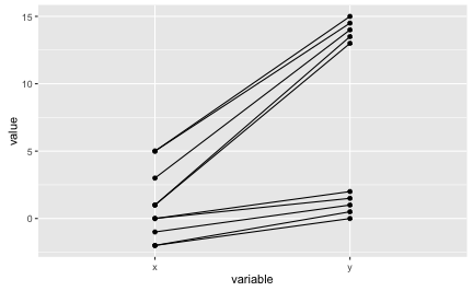
Ordinal association is perfect if the ranking in both variables is identical. Let’s visualize ordinal association. Visually, as in the following diagram, this amounts to non-intersecting lines:
library(tidyr)

df_long <- tidyr::gather(df, key = variable, value = value, -ID)
# df_long

ggplot(df_long, aes(x = variable, y = value)) + geom_point() +
  geom_line(aes(group = ID))

As can be seen in the diagram above, the lines are not intersecting. So the ordinal association measures should be (close to) 1. Actually, we have some ties, that’s why our measures (Spearman, Kendall) are not perfectly one. Note that the raw value are depicted.
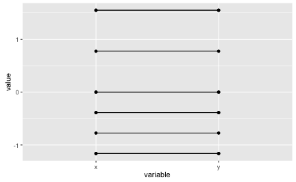
Now let’s visualize Pearson correlation. Pearson’s r can be seen as a function of the z-values, so let’s depict z-values of a perfect correlation as a first step.
df_z <- data.frame(scale(df))
df_z$ID <- 1:10
df_z$y <- df_z$x

df_z_long <- gather(df_z, key = variable, value = value, -ID)
ggplot(df_z_long, aes(x = variable, y = value)) + geom_point() +
  geom_line(aes(group = ID))

Perfect correlations amounts to horizontal lines in our diagram (remember that z-values are used instead of raw values.) Now let’s look at our example data in the next step.
df_z <- data.frame(scale(df))
df_z$ID <- 1:10
df_z_long <- gather(df_z, key = variable, value = value, -ID)


# df_z_long
ggplot(df_z_long, aes(x = variable, y = value)) + geom_point() +
  geom_line(aes(group = ID))

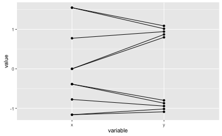
The lines are far from being horizontal. The z-values are quite different between the two variables as can be seen in the diagram. But still, Pearson’s r is very high. We must infer that strong ordinal assocation is enough to get r really high.
We see that a high r does not guarantee that the z-values between the two variables are similar. Similarly, if both the ordinal association measure (Spearman, Kendall) and the metric association measure (Pearson r) are high, we cannot infer that the metric values and the ranks are identical or very similar.
That’s why I emphatically insist that e.g., Labovitz 1970 is outright wrong when he argues that r and rho yields similar numbers, hence, ordinal can be taken as metric.