Load packages

library(tidyverse)
library(mosaic)

We are following here the advise of Gelman and Hill (2007, p. 46-47).

Validity

Quite obviously, the right predictors must be included in the model in order to learn something from the model. The “right” predictors means: avoiding the wrong ones, and including the correct ones. Easier said than done, particularly with a look to the causal inference aspects. Let’s turn to the next most important assumption.

Additivity and linearity as the second most important assumptions in linear models

We assume that \(y\) is a linear function of the predictors. If y is not a linear function of the predictors, we cannot expect the model to deliver correct insights (predictions, causal coefficients). Let’s check an example.

Simulate an exponentially distributed assocation

We will only use positive values, let’s add some small value to the y’s in order they are all positive.

len <- 42  # 42 x values
set.seed(42)
x <- rep(runif(len), 30)  # each x value repeated 30 times
y <- dexp(x, rate = 5) + rnorm(length(x), mean = 0, sd = .1)  # add some noise

y <- y + 1
gf_point(y ~ x)

Linear model

Compute the Model as linear model (not transformed)

lm1 <- lm(y ~ x)
coef(lm1)
#> (Intercept)           x 
#>    3.797730   -3.458985

Plot it

gf_point(y ~ x) %>% 
  gf_abline(slope = coef(lm1)[2], intercept = coef(lm1)[1], color = "red")

Doesn’t fit well.

Check the linearity assumption

Actually the plot above vividly shows us that the linear model is not doing a good job. But anyhow, let’s put that in a form more typically used for checking model assumptions.

gf_point(lm1$residuals ~ fitted(lm1)) %>% 
  gf_smooth() %>% 
  gf_lims(y = c(-3, 3))

If we had a linear trend, we should see no strong pattern whatsoever. The mean residual should jump around zero at each value of the x-axis, with the variance remaining (more or less) constant. This is not the case here.

Second model: log-tranformed in y

gf_point(log(y) ~ x)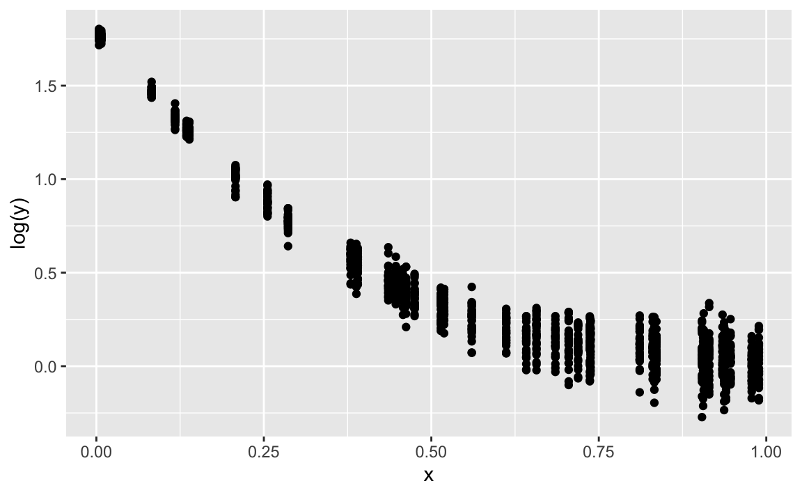

lm2 <- lm(log(y) ~ x)
coef(lm2)
#> (Intercept)           x 
#>    1.331698   -1.556101

gf_point(log(y) ~ x) %>% 
  gf_abline(slope = coef(lm2)[2], intercept = coef(lm2)[1], color = "red")

Quite ok. Note that the discrepancies stem completely from the fact that we added some Gaussian noise.

gf_point(resid(lm2) ~ fitted(lm2)) %>% 
  gf_smooth() %>% 
  gf_lims(y = c(-3, 3))

Much better than the first model.

Most important asssumption in linear models ... and the second most